Changing Number Display Settings for Single Workbooks

Allen is a Canadian Excel user who often downloads large amounts of statistical data from European sources, thereby experiencing the usual problems with decimals and thousands separators being reversed. This requires some fancy manipulation to change to North American style and often results in mistakes. Allen could change the settings on his entire system, but then his North American numbers (in other workbooks) are screwed up. He wonders if there is some way to change just one file at a time.

How numbers are displayed depends on the Regional Settings maintained in Windows. If you change the Regional Settings, then Excel adopts those settings and displays information differently. So, for instance, if I create a workbook here in the United States, and someone opens that workbook in a location that uses different Regional Settings, then they will see my numbers according to their Regional Settings, not according to the settings of the United States.

If this is not happening, then it could be that the person who created the workbook configured Excel to ignore the Regional Settings. You can do that in this manner:

1. Display the Excel Options dialog box. (In Excel 2007 click the Office button and then click Excel Options. In Excel 2010 and later versions display the File tab of the ribbon and then click Options.)
2. At the left side of the dialog box click Advanced.
3. Scroll down until you see the Editing Options section. (See Figure 1.) (You shouldn't have to scroll far; this section is the first one in this part of the dialog box.)



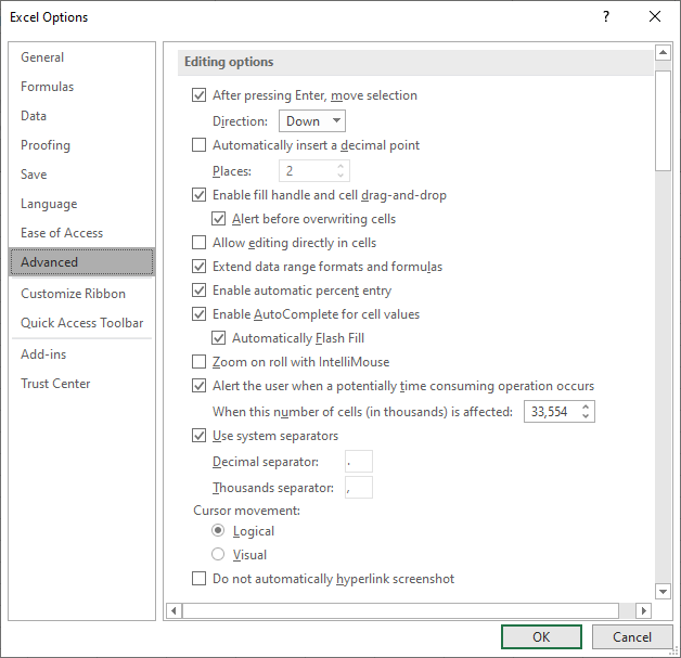
Figure 1. The Editing Options settings in Excel.

Note the setting of the Use System Separators check box. If this check box is selected (which it is by default), then Excel uses the settings maintained in Windows' Regional Settings area. If you clear this check box, then Excel will use whatever characters you specify in the Decimal Separator and Thousands Separator boxes.

If you want to modify the separators on a workbook by workbook basis (as Allen apparently wants to do), then the easiest way is to use a macro. For instance, the following event-handler macros, when included in the ThisWorkbook module, will change these settings whenever you make the workbook active.

Private Sub Workbook_Activate()
    Application.DecimalSeparator = ","
    Application.ThousandsSeparator = "."
    Application.UseSystemSeparators = False
End Sub

Private Sub Workbook_Deactivate()
    Application.UseSystemSeparators = True
End Sub

Note that the macro changes the decimal and thousands separators and then clears the Use System Separators setting. When the workbook is left (when a different workbook receives focus), then the Use System Separators setting is again set.

If you prefer to change information on the fly rather than automatically, you could use this quick little macro. When you assign it to the Quick Access Toolbar you can click it to switch between two different sets of separator values.

Sub ToggleSep()
    Dim bCurrent As Boolean

    bCurrent = Application.UseSystemSeparators
    If bCurrent Then
        Application.DecimalSeparator = ","
        Application.ThousandsSeparator = "."
        Application.UseSystemSeparators = False
    Else
        Application.UseSystemSeparators = True
        MsgBox "Now Using System Separators"
    End If
End Sub

The macro displays a message when it "returns" to the default of using the system separators defined within Windows.

You should note that everything discussed in this tip assumes that any cells containing numbers are not formatted with some custom format that overrides how Excel uses the separators. Any custom formats always take precedence. Thus, if you see no change after adjusting the separators used by Excel, then you'll want to check to see how the actual cells are formatted.

ExcelTips is your source for cost-effective Microsoft Excel training. This tip (13453) applies to Microsoft Excel 2007, 2010, 2013, 2016, 2019, Excel in Microsoft 365, and 2021.