Written by Allen Wyatt (last updated November 29, 2022)
This tip applies to Excel 2013, 2016, 2019, and 2021
Feroz has a series of text values in column A. These values are formatted with two different font colors in each cell. (First part of text is one color and the second part is a different color.) He would like to split these text values into columns B and C, such that anything with the first color is in column B and anything with the second color is in column C. He notes that the Text to Columns tool won't handle this, so he wonders if it can be done.
Yes, it can be done. One way is to use Excel's built-in Flash Fill capability. (This tool is available only in Excel 2013 or later versions.) Let's say you are starting with data that looks like this: (See Figure 1.)
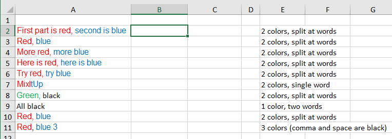
Figure 1. Your multi-colored data.
Note that my testing data includes, in column E, some characteristics of the data in column A. At this point, all you need to do is to give Flash Fill something it can work with. I do this by manually breaking apart the text in rows 2 and 3, as shown here: (See Figure 2.)
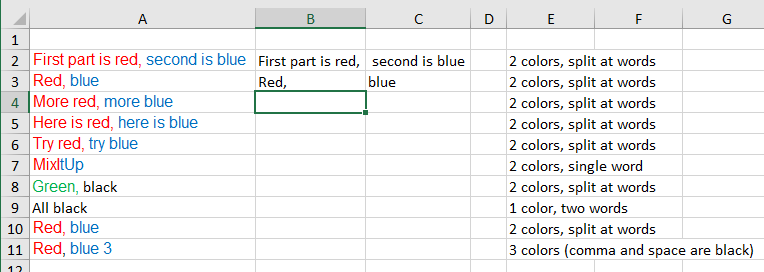
Figure 2. Setting up the examples.
It is important that the examples you create in B2:C3 are exact—they should include anything that is in whatever color (including leading or trailing spaces) and both spelling and capitalization should be correct.
Now select cell B4 and press Ctrl+E. This makes Flash Fill spring into action, and you will see in text appear in the rest of column B. Do the same thing in column C—select cell C4 and press Ctrl+E. Your results should look similar to the following: (See Figure 3.)
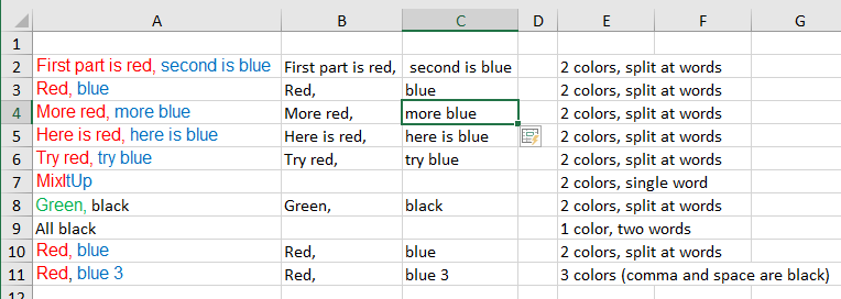
Figure 3. After using Flash Fill in both columns.
I should note that your success with Flash Fill will depend, in large part, on the characteristics of the data in column A. It will, in most cases, do the majority of the work, and it may complete the task tremendously. There may be some strange instances in which Flash Fill cannot discern how it should pull apart your data. You can see this in the previous figure where cells A7, A9, and A11 were not pulled apart correctly. You'll want to check your results carefully to make sure they make sense.
If Flash Fill doesn't work for you, then you will want to create a macro to do the work. It is possible to come up with a macro that will work on all the cells in column A and pull the text into columns B and C (like Feroz needs), but it is more flexible to create a user-defined function that will return whatever is wanted from the cell. Here's an example:
Function SplitColors(r As Range, Optional iWanted As Integer = 1) _
  As String
    Dim sTemp As String
    Dim J As Integer
    Dim K As Integer
    Dim iColors(9) As Integer

    sTemp = ""
    If r.Cells.Count = 1 Then
        For J = 1 To 9
            iColors(J) = 0
        Next J

        ' Determine where colors change
        ' Remember there will always be at least one color
        K = 1
        iColors(K) = 1
        For J = 2 To Len(r.Text)
            If r.Characters(J,1).Font.Color <> _
              r.Characters(J-1,1).Font.Color Then
                K = K + 1
                iColors(K) = J
            End If
        Next J

        ' Check if wanted color is less than total colors
        If iWanted <= K Then
            J = iColors(iWanted + 1)
            If J = 0 Then J = Len(r.Text) + 1
            J = J - iColors(iWanted)
            sTemp = Mid(r.Text, iColors(iWanted), J)
        End If
    End If
    SplitColors = sTemp
End Function
The SplitColors function requires one parameter (a range to act upon) and a second, optional parameter (which color from the range you want). The function checks, first, to see if it was passed a single cell. If so, then it determines how many colors are in that cell and the character numbers where the color changes occur. Then, if the desired color (passed in the optional second parameter) is less than the number of colors in the cell, the characters using that color are returned.
So, for instance, if you want to return the cells using the first color in cell A2, you could use either of the following in your worksheet:
=SplitColors(A2, 1)
=SplitColors(A2)
The second invocation works because the second parameter is optional. If you do not include it, then the function assumes you want to work with the first color. If you want to return the text using the second color in the cell, then the following will work:
=SplitColors(A2, 2)
The SplitColors function will work with up to 9 colors in whatever cell you are checking out. If you specify a second parameter of 9 or greater, then you'll end up with an error.
Note:
ExcelTips is your source for cost-effective Microsoft Excel training. This tip (13605) applies to Microsoft Excel 2013, 2016, 2019, and 2021.

Program Successfully in Excel! This guide will provide you with all the information you need to automate any task in Excel and save time and effort. Learn how to extend Excel's functionality with VBA to create solutions not possible with the standard features. Includes latest information for Excel 2024 and Microsoft 365. Check out Mastering Excel VBA Programming today!
If you only want to import a portion of whatever records are in a text file, Excel provides a number of ways you can ...
Discover MoreAt the very heart of editing is the ability to move and copy cells in a worksheet. Understanding the differences between ...
Discover MoreNeed to get rid of everything in a worksheet except for your formulas? You can do it rather easily by applying the ideas ...
Discover MoreFREE SERVICE: Get tips like this every week in ExcelTips, a free productivity newsletter. Enter your address and click "Subscribe."
2019-01-10 06:07:03
Harold Druss
Peter
This solves MixItUp:
With Application
str1 = Trim(Left(c, I - 1))
str2 = Trim(Right(c, L - (I - 1)))
End With
2019-01-09 16:53:58
Yvan Loranger
I was expecting when I 1st read Feroz's question he meant data like in row7 [ie MixItUp with 1st part 1 colour & 2nd part a diff. colour].
2019-01-08 18:36:27
Yvan Loranger
The dataset presented in Allen's Tip can be totally solved by Text to Columns [& then reinserting the comma (lost by delimiting by comma) at end of column B, and another trivial cosmetic fix].
2019-01-06 10:22:27
Peter Atherton
I lost the picture
[fig}]
2019-01-06 10:14:17
Peter Atherton
John
I think that you are right, it splits on spaces or maybe commas. This is the nearest I can get but it does not work in a word with separate colours. Here is the closest I can get. It fails on MixItUp when miedCololours are used Unlike Allen's function, but it does split two colours.
Sub SplitIt()
Dim c As Range, I As Integer, L As Integer, _
myColour As Long, FontName As String, _
str1 As String, str2 As String
For Each c In Selection
str1 = "": str2 = ""
c.Select
L = Len(c)
With c
myColour = .Characters(1, 1).Font.Color
FontName = .Characters(1, 1).Font.Name
For I = 2 To L
If .Characters(I, 1).Font.Color <> myColour Or _
.Characters(I, 1).Font.Name <> FontName Or _
.Characters(I, 1).Font.Color = 0 Then
With Application
str1 = Trim(Left(c, I))
str2 = Trim(Right(c, L - I))
End With
c.Offset(0, 1).Value = str1
c.Offset(0, 2).Value = str2
Exit For
End If
Next
End With
Next
End Sub
[{fig.}]
2019-01-06 09:02:05
If Feroz does not have Excel 2013 this will do what Feroz wants.
Split each cell in Col A by text color and put results in Col B and Col C.
=============================================================
Sub SplitByColor2()
Dim strFirstSection As String ' holds the text that has the first color
Dim i As Integer ' loop through each character in a cell
Dim LastRow As Integer
Dim J As Integer ' loops through each row
Dim iFontColor As Long, iFontColor2 As Long
' get the last row in column A that has data
LastRow = Cells(Rows.Count, "A").End(xlUp).Row
' loop through each character in the cell until font color changes
For J = 1 To LastRow
' font color of the first character in the cell
iFontColor = Range("A" & J).Characters(1, 1).Font.Color
' font color of last character in the cell
iFontColor2 = Range("A" & J).Characters(Len(Range("A" & J).Text), 1).Font.Color
' loop through the cel(Aj) and check each character for it's font color
For i = 1 To Len(Range("A" & J).Value)
If Range("A" & J).Characters(i, 1).Font.Color = iFontColor Then
strFirstSection = strFirstSection & Mid(Range("A" & J).Value, i, 1)
Else ' font color has changed
Exit For
End If
Next
Range("B" & J).Value = Trim(strFirstSection)
Range("B" & J).Select
Selection.Font.Color = iFontColor
Range("C" & J).Value = Trim(Mid(Range("A" & J).Value, Len(strFirstSection) + 1))
Range("C" & J).Select
Selection.Font.Color = iFontColor2
' reset for next cell ("A" & J)
strFirstSection = ""
Next
End Sub
=====================================================================
2019-01-05 22:03:32
John Plant
A third, hopefully clearer example
(see Figure 1 below)
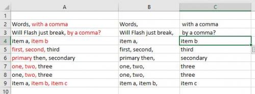
Figure 1.
2019-01-05 21:57:44
John Plant
Sorry. This is a better example showing that the comma(s) is the separator used despite colors.
(see Figure 1 below)
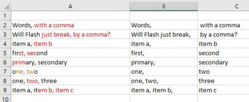
Figure 1.
2019-01-05 21:39:25
John Plant
I had a play with this and seems to me that Flash Fill breaks on the commas and pays no attention to the colours at all.
(see Figure 1 below)
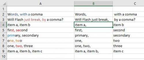
Figure 1.
2019-01-05 21:32:40
John Plant
I had a play with this and seems to me that Flash Fill breaks on the commas and pays no attention to the colours at all.
Got a version of Excel that uses the ribbon interface (Excel 2007 or later)? This site is for you! If you use an earlier version of Excel, visit our ExcelTips site focusing on the menu interface.
FREE SERVICE: Get tips like this every week in ExcelTips, a free productivity newsletter. Enter your address and click "Subscribe."
Copyright © 2025 Sharon Parq Associates, Inc.
Comments