Importing a Subset of Records

Gordon wonders how he can import a subset of a text file into Excel, depending upon the value of a particular field. As an example, he may want to only import records that contain a "y" in column 5 of each record in the text file.

There are several ways you can approach this task. One is that you could simply import the whole text file, sort the records, and delete those you don't want. This is, perhaps, the simplest option if you only need to process a single file and the entire file can fit within a single worksheet.

Another approach is to use a macro. (This is the one that I find the fastest and easiest, particularly if you need to import the same type of file quite a bit.) The macro can open the text file, read each line, and then make a determination as to whether the information in that line should be added to the worksheet or not. Here's an example that will open a file named "MyCSVFile.txt" and then stick the data into a new worksheet starting at the first row.

Sub ReadMyFile()
    Dim R As Integer
    Dim C As Integer
    Dim sDelim As String
    Dim sRaw As String
    Dim ReadArray() As String

    sDelim = ","     ' Set to vbTab if tab-delimited file

    Worksheets.Add
    Open "myCSVFile.txt" For Input As #1
    R = 1
    Do While Not EOF(1)
        Line Input #1, sRaw
        ReadArray() = Split(sRaw, sDelim, 20, vbTextCompare)
        If ReadArray(4) = "y" Then
            For C = 0 To UBound(ReadArray)
                Cells(R, C + 1).Value = ReadArray(C)
            Next C
            R = R + 1
        End If
    Loop
    Close #1
End Sub

To use the macro, simply change the name of the file to match the file you want to process. You'll also want to modify the sDelim variable to make sure it matches whatever is being used as a delimiter in your records. As written, it assumes the delimiter is a comma (which it would be in a CSV file), but you could change it to vbTab if you are actually working with a tab-delimted file. After the macro is complete, only those records with a single, lowercase "y" character are in the new worksheet.

Another approach is to use the Power Query feature of Excel. This is a free add-in, from Microsoft, that is available for some variations of Excel 2010 and Excel 2013. You can download (and find out which variations are supported) at this location:

http://www.microsoft.com/en-us/download/details.aspx?id=39379

If you are using Excel 2016, then Power Query is built into the program. If you have Power Query installed or available in your version of Excel and that version of Excel happens to be Excel 2010 or Excel 2013, then follow these steps:

1. Display the Power Query tab of the ribbon.
2. Click From File | From CSV. Excel displays the Comma-Separated Values Browse dialog box, which looks very much like a standard Open dialog box.
3. Locate and select the CSV file you want to import into Excel.
4. Click Open. Excel loads the data in a Power Query window with filtering buttons available for each field.

If you are using Excel 2016 or a later version, the steps are a bit different:

1. Display the Data tab of the ribbon.
2. Click the New Query tool (Excel 2016) or the Get Data tool (later versions of Excel) in the Get & Transform group. Excel displays some options.
3. Click From File | From Text/CSV. Excel displays the Import Data dialog box, which looks very much like a standard Open dialog box.
4. Locate and select the CSV file you want to import into Excel.
5. Click Open. Excel loads the data in a Power Query window with filtering buttons available for each field.

At this point—regardless of the version of Excel you are using—you can use the controls to specify a query (meaning, setting up a definition of which records should be imported). When you click Close and Load, the records are retrieved from the file, and the query can be saved for future use.

A fourth approach is to use Microsoft Query. To do so, you'll need to follow this very lengthly series of steps. (Nobody ever said that Microsoft wanted to make Microsoft Query easy to use, and you'll agree after you go through these steps.)

1. Display the Data tab of the ribbon.
2. Click the Get Data tool in the Get & Transform Data group, then choose From Other Sources (in the Get External Data group earlier versions of Excel) and then choose From Microsoft Query. Excel displays the Choose Data Source dialog box. (See Figure 1.)



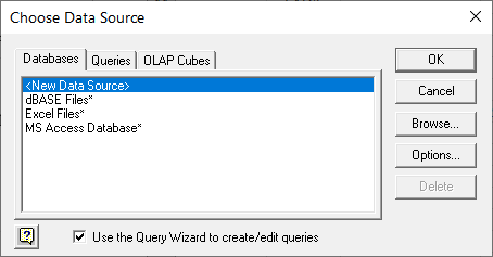
Figure 1. The Choose Data Source dialog box.

3. Select the New Data Source option and click OK. Excel displays the Create New Data Source dialog box. (See Figure 2.)



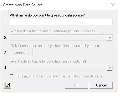
Figure 2. The Create New Data Source dialog box.

4. Provide a name for your data source, such as "CSV Files".
5. Using the drop-down list for item 2, choose Microsoft Text Driver.
6. Click Connect. Excel displays the ODBC Text Setup dialog box.
7. Immediately click OK to close the dialog box.
8. Click OK to close the Create New Data Source dialog box. Excel updates the Choose Data Source dialog box to include the name you specified in step 4.
9. Select the data source you just created and then click OK. Excel displays a warning that there are no data tables in the source. (That's OK; you haven't defined any.)
10. Click OK to dismiss the warning. Excel displays the Query Wizard dialog box.
11. Since you can't do anything with an empty Query Wizard dialog box, click Cancel. Excel displays a warning asking if you want to remain in Microsoft Query.
12. Click Yes. Excel displays the Add Table dialog box.
13. Using the controls in the dialog box, locate and select your CSV file.
14. Click the Add button. Excel looks like it doesn't do anything, but it actually added the reference to the CSV file.
15. Click the Close button to dismiss the Add Table dialog box. Your CSV file is shown in the Microsoft Query window.
16. Using the list of fields for the CSV file, drag each field you want imported into the worksheet into the bottom area of the Microsoft Query window. (If you want all of the fields, just drag the asterisk into the bottom area of the window.)
17. Click Criteria | Add Criteria. Excel displays the Add Criteria dialog box. (See Figure 3.)



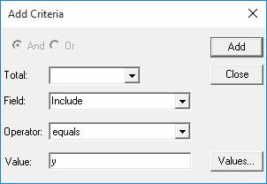
Figure 3. The Add Criteria dialog box.

18. Using the controls in the dialog box, specify that you want field 5 (whatever its name is) to be equal to "y."
19. Click the Add button to actually add the criteria to the query.
20. Click Close to dismiss the Add Criteria dialog box.
21. Click File | Return Data to Microsoft Excel. Excel displays the Import Data dialog box. (See Figure 4.)



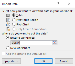
Figure 4. The Import Data dialog box.

22. Change the settings in the dialog box, as desired, to indicate how you want the CSV data returned to Excel.
23. Click OK.

(Told you the steps were lengthly.) You can now work with the data in Excel and, if desired, use the tools on the Design tab of the ribbon to refresh the data from the CSV file.

ExcelTips is your source for cost-effective Microsoft Excel training. This tip (10384) applies to Microsoft Excel 2007, 2010, 2013, 2016, 2019, Excel in Microsoft 365, and 2021.