Quickly Adding Formulas Referencing Multiple Worksheets

Tyler has a workbook with a Trends worksheet followed by a worksheet for each day of the year. He needs to populate the Trends worksheet with data from every other worksheet. The cell needed is constant within each sheet. Tyler wonders how he can grab that data without manually doing "=A23" for each of the 365 worksheets.

There are a couple of ways you can approach this task, depending on exactly what you want to do. If you just want to get a sum for all of the 365 worksheets, you could use a formula such as the following:

=SUM('Day1:Day365'!A23)

This assumes that your worksheets are named Day1 through Day365. An easy way to remove all doubt, however, is to follow these steps:

1. Select the cell in the Trends worksheet where you want to enter your formula.
2. Start to type in the formula: =SUM(
3. Click on the first worksheet tab (the one for the first day).
4. Hold down the Shift key as you click on the last worksheet tab (the one for the last day). Your formula should now look similar to this: =SUM('Day1:Day365'!
5. Click the cell you want summed, in this case cell A23. (It doesn't matter which worksheet you do this on.) Your formula will now look similar to this: =SUM('Day1:Day365'!A23
6. Press Enter. This finishes out the formula for you.

Of course, you may not want to sum a cell across worksheets. You may, in fact, simply want to list all 365 values in the Trends worksheet. In that case, the easiest method is to list all of the worksheet names just to the left of where you want the values listed. For instance, you might include all the worksheet names in column A. You can then use the INDIRECT function in a formula in column B:

=INDIRECT("'"&A7&"'!A23")

Copy this down as many cells as necessary, and you end up with the desired values pulled from those other worksheets into column B. (See Figure 1.)

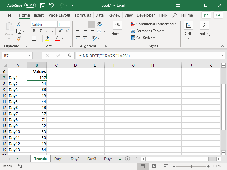
Figure 1. Pulling values into the Trends worksheet.

You can do away with the worksheet names in column A if you make sure your worksheets are named with some sort of pattern. For instance, you might have them named something like "Jan 01" through "Dec 31". In that case, you just modify the formula in column B, to something like this:

=INDIRECT("'"& TEXT(DATE(2019,1,ROW()-6), "mmm dd")&"'!A23")

Copy the formula down as many cells as necessary, and you have the values you want. (See Figure 2.)

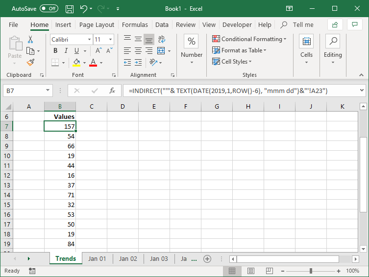
Figure 2. Pulling values into the Trends worksheet using dates.

Note that the formula subtracts 6 from what the ROW function returns because it is being entered into cell B7. If you are actually putting this formula into a different row, you'll want to adjust what you actually subtract.

ExcelTips is your source for cost-effective Microsoft Excel training. This tip (6089) applies to Microsoft Excel 2007, 2010, 2013, 2016, 2019, 2021, 2024, and Excel in Microsoft 365.