Conditional Formatting for Errant Phone Numbers

If you use Excel to store a list of phone numbers, you may want a way to determine if any of the phone numbers in your list are outside of a specific range. For instance, for your area, only phone numbers in the 240 exchange (those beginning with 240) may be local calls. You might want to highlight all the phone numbers in the list that do not begin with 240, and therefore would be long distance.

The way that you do this depends on whether your phone numbers are stored as text or as formatted numbers. If you enter a phone number with dashes, periods, parentheses, or other non-numeric characters, then the phone number is considered a text entry. If you format the cells as phone numbers (Format Cells dialog box | Number tab | Special | Phone Number), then the phone number is considered a number and formatted for display by Excel.

If your phone numbers are text entries, then use these steps to apply the desired conditional formatting:

1. Select the cells containing the phone numbers. (For the sake of this example, I assume that the first cell you select is A3.)
2. With the Home tab of the ribbon displayed, click the Conditional Formatting option in the Styles group. Excel displays a palette of options related to conditional formatting.
3. Click New Rule. Excel displays the New Formatting Rule dialog box. (See Figure 1.)



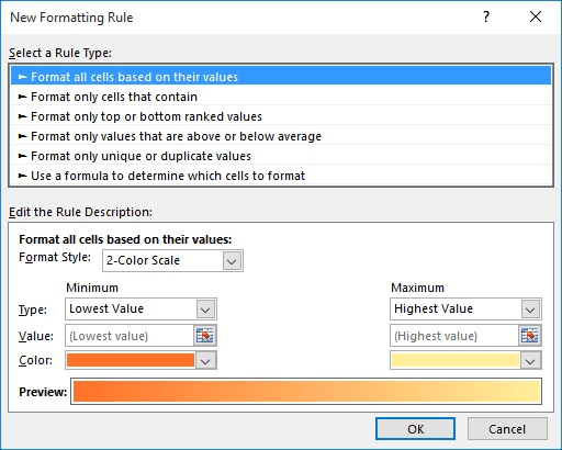
Figure 1. The New Formatting Rule dialog box.

4. In the Select a Rule Type area at the top of the dialog box, choose Use a Formula to Determine Which Cells to Format.
5. In the Format Values Where This Formula Is True box, enter the following formula, replacing A3 with the address of the active cell selected in step 1:

     =LEFT(A3,3)<>"240"

6. Click Format to display the Format Cells dialog box.
7. Set the formatting options to highlight the errant phone numbers, as desired.
8. Click OK to dismiss the Format Cells dialog box. The formatting you specified in step 7 should now appear in the preview area for the rule.
9. Click OK.

These steps will even work if the phone numbers are numeric, but you may want to use a different approach if the phone numbers were entered as numbers. The following steps will work:

1. Select the cells containing the phone numbers. (For the sake of this example, I assume that the first cell you select is A3.)
2. With the Home tab of the ruler displayed, click the Conditional Formatting option in the Styles group. Excel displays a palette of options related to conditional formatting.
3. Click New Rule. Excel displays the New Formatting Rule dialog box.
4. In the Select a Rule Type area at the top of the dialog box, choose Format Only Cells That Contain. The left portion of the rule description should automatically be set to Cell Value.
5. Use the next drop-down list in the rule description to choose Not Between.
6. Set the lower and upper boundaries of the condition to 2400000 and 2409999, respectively. (You are specifying that the condition is met if the number is not between 2400000 and 2409999, which is the range of acceptable phone numbers.) (See Figure 2.)



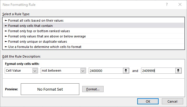
Figure 2. The New Formatting Rule dialog box.

7. Click Format to display the Format Cells dialog box.
8. Set the formatting options to highlight the errant phone numbers, as desired.
9. Click OK to dismiss the Format Cells dialog box. The formatting you specified in step 8 should now appear in the preview area for the condition.
10. Click OK.

If you want to convert your textual phone numbers to numeric phone numbers, so that you can use this last method of conditional formatting, you need to "clean up" your list of numbers. In other words, you need to remove all non-numeric characters from the phone numbers. You can do this using Find and Replace to repeatedly remove each non-numeric character, such as dashes, periods, parentheses, etc. Once the phone numbers are clean, you can format them as phone numbers (using the Format Cells sequence mentioned earlier in this tip) and use the conditional formatting just described.

ExcelTips is your source for cost-effective Microsoft Excel training. This tip (6178) applies to Microsoft Excel 2007, 2010, 2013, 2016, 2019, and Excel in Office 365. You can find a version of this tip for the older menu interface of Excel here: Conditional Formatting for Errant Phone Numbers.