Applying Table Formats

At times formatting can be rather tedious, particularly if your worksheet is large or presents complex information. Excel includes a very powerful formatting tool that you can use to help with your formatting tasks. This is the table formatting feature, which allows you to format data tables within your worksheet quickly and easily. With the click of a mouse button, you can format an entire table, including setting all formatting attributes and row and column sizes.

To use this feature, simply make sure you select a cell in or around a data table. When you select a cell within the data table, AutoFormat does real good at just selecting the cells that make up the data table. However, if you choose a cell around the data table (within one row or column of the data table), AutoFormat selects the entire data table plus the extra row or column that contains the cell you selected. If you want to format only the data table and no extra rows or columns, you will want to make sure the cell you select is actually within the data table.

Once you have selected a cell (or the entire data table), follow these steps:

1. Display the Home tab of the ribbon.
2. In the Styles group, click Format As Table. Excel displays a palette of available table styles.
3. From the available styles, click on the style that looks like how you want your data to look. Excel displays the Format As Table dialog box. (The range for your table should already be filled in.) (See Figure 1.)



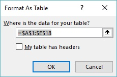
Figure 1. The Format As Table dialog box.

4. Click OK. Excel reformats your table to match the format you selected.

ExcelTips is your source for cost-effective Microsoft Excel training. This tip (6256) applies to Microsoft Excel 2007, 2010, 2013, 2016, 2019, Excel in Microsoft 365, and 2021. You can find a version of this tip for the older menu interface of Excel here: Applying Table Formats.