Please Note: This article is written for users of the following Microsoft Excel versions: 2007, 2010, 2013, 2016, 2019, and 2021. If you are using an earlier version (Excel 2003 or earlier), this tip may not work for you. For a version of this tip written specifically for earlier versions of Excel, click here: Controlling the Plotting of Empty Cells.
When you create a chart from a data table, Excel does its best to translate the numeric values into data points on a chart, according to the specifications you provide. One area where Excel doesn't quite know what to do, however, is empty cells. If a cell is empty, it could be for any number of reasons—the value isn't available, the value isn't important, or the value is really zero.
You can instruct the program how you want it to treat empty cells by following these steps:
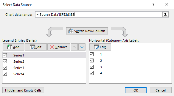
Figure 1. The Select Data Source dialog box.
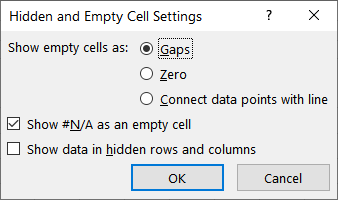
Figure 2. The Hidden and Empty Cell Settings dialog box.
The option buttons at the top of the Hidden and Empty Cell Settings dialog box (step 5) provide the following three settings:
ExcelTips is your source for cost-effective Microsoft Excel training. This tip (6289) applies to Microsoft Excel 2007, 2010, 2013, 2016, 2019, and 2021. You can find a version of this tip for the older menu interface of Excel here: Controlling the Plotting of Empty Cells.

Professional Development Guidance! Four world-class developers offer start-to-finish guidance for building powerful, robust, and secure applications with Excel. The authors show how to consistently make the right design decisions and make the most of Excel's powerful features. Check out Professional Excel Development today!
Excel makes it easy to copy charts from one workbook to another. Even so, copying may produce some surprising results for ...
Discover MoreExcel allows you to create all sorts of charts to visually display your data. With so many options available, how do you ...
Discover MoreWhen creating a chart, you may want to adjust the default scaling that Excel applies to an axis. This is relatively easy ...
Discover MoreFREE SERVICE: Get tips like this every week in ExcelTips, a free productivity newsletter. Enter your address and click "Subscribe."
There are currently no comments for this tip. (Be the first to leave your comment—just use the simple form above!)
Got a version of Excel that uses the ribbon interface (Excel 2007 or later)? This site is for you! If you use an earlier version of Excel, visit our ExcelTips site focusing on the menu interface.
FREE SERVICE: Get tips like this every week in ExcelTips, a free productivity newsletter. Enter your address and click "Subscribe."
Copyright © 2026 Sharon Parq Associates, Inc.
 Please Note:
This article is written for users of the following Microsoft Excel versions: 2007, 2010, 2013, 2016, 2019, and 2021. If you are using an earlier version (Excel 2003 or earlier), this tip may not work for you. For a version of this tip written specifically for earlier versions of Excel, click here:
Please Note:
This article is written for users of the following Microsoft Excel versions: 2007, 2010, 2013, 2016, 2019, and 2021. If you are using an earlier version (Excel 2003 or earlier), this tip may not work for you. For a version of this tip written specifically for earlier versions of Excel, click here:
Comments