Leaving a Cell Value Unchanged If a Condition Is False

While using the IF function, Vineet wants to retain the old value in the cell if the condition is false. In other words, the value in a cell where the IF function is used should change only if the condition being tested by the IF function is true. By default, however, the IF function makes the value 0 if the condition is False.

The IF function can take up to three parameters. The first parameter is the comparison that is to be made, the second parameter is what should be returned if the comparison is true, and the third is what should be returned if the comparison is false. It is possible to leave off the last parameter, but if you do then Excel will return the value 0 if the comparison is false. (This is what Vineet is seeing returned by his IF function usage.)

The obvious solution, then, is to make sure that you provide the IF function with something that should be returned when the comparison is false. For instance, let's say that your formula is in cell B1 and you are comparing something in cell A1. The formula you use may look like this:

=IF(A1<10,"under ten",B1)

Note that the words "under ten" are returned if the value in A1 is less than 10. If this condition is not met, then the value in B1 is returned. Since this formula is in cell B1, this means that the previous value in the cell is returned if the condition is false.

It also means that the formula contains a circular reference. For circular references to work OK you need to let Excel know that it is OK for them to occur in your worksheet. Follow these steps if you are using Excel 2010 or a later version:

1. Display the File tab of the ribbon and then click Options. Excel displays the Excel Options dialog box.
2. At the left side of the dialog box, choose Formulas. (See Figure 1.)



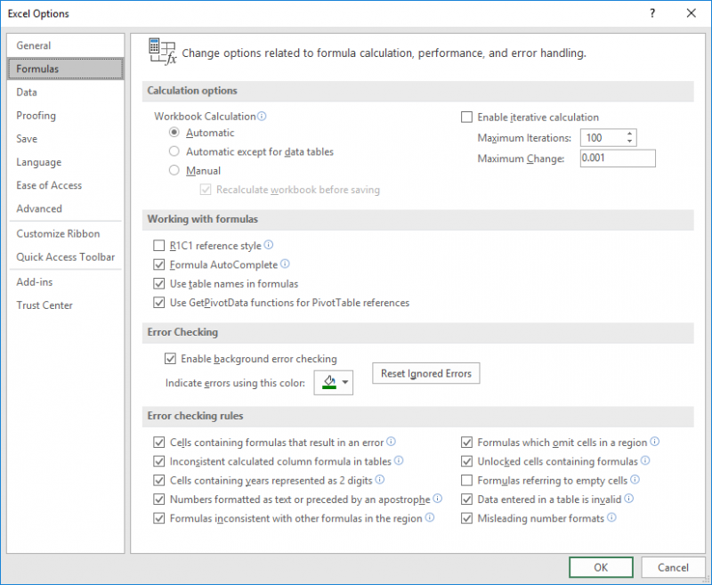
Figure 1. The Formulas tab of the Excel Options dialog box.

3. Make sure the Enable Iterative Calculation check box is selected.
4. Click OK.

If you are using Excel 2007, choose Tools | Options | Calculation tab and make sure the Iteration check box is selected. Excel will now allow the circular reference without complaint.

If you don't want to allow a circular reference in your worksheet, then the only recourse is to create a macro that updates the value in cell B1 based upon any changes to cell A1:

Private Sub Workbook_SheetChange(ByVal Sh As Object, _
  ByVal Target As Range)

    ' See if the change is related to our cell
    If Not (Application.Intersect(Target, Range("A1")) _
      Is Nothing) Then
        If Range("A1") < 10 Then
            Range("B1") = "under ten"
        End If
    End If
End Sub

This simple macro, when added to the ThisWorkbook module, is executed every time there is a change in the workbook. If the value is cell A1 is changed (and only that cell), then the value is checked to see if it is less than 10. If it is, then the value in cell B1 is changed. If it isn't, then the value in cell B1 is left alone.

There is one "gotcha" that you need to keep in mind with any of the approaches discussed thus far, formula or macro. If the value in cell A1 is (let's say) 15, then cell B1 will contain what was there before, whatever it was. If you change the value in cell A1 to (let's say) 7, then B1 will change to "under ten." That's fine, but from that point on cell B1 will never appear to change. Why? Because if you then change cell A1 to a value greater than 10, cell B1 will contain (as just explained) what was there before. And, as you now understand, the value that was there before is the result of the previous true result, which was "under ten." Thus, true or false, the formula or macro from this point on displays the text "under ten."

ExcelTips is your source for cost-effective Microsoft Excel training. This tip (8264) applies to Microsoft Excel 2007, 2010, 2013, 2016, 2019, and Excel in Microsoft 365. You can find a version of this tip for the older menu interface of Excel here: Leaving a Cell Value Unchanged If a Condition Is False.