Greg knows he can use filtering to display just a subset of rows in a worksheet. He would like, in an unused column, to sequentially number the rows that are visible after filtering. He can use AutoFill to number unfiltered rows, but he wants to number just the visible, filtered rows.
The simple, traditional way to do this is to add a formula to the unused column before you apply your filter. For example, let's say that the values on which you are going to filter are in column A, beginning in cell A3, and that your unused column is F. Then, in cell F3 you should enter the following formula:
=SUBTOTAL(103,$A$3:A3)
Copy this formula down as many cells as necessary. The formula should show a count for each item visible in column A. When you apply your filter, the formulas are updated to display a count for each filtered row.
As simple as this is, it does have a drawback: If you remove the filter, then the formula is updated to number (again) the visible rows. If, however, you had wanted the numbers to remain on the cells corresponding to the rows that had been previously filtered, then the SUBTOTAL approach won't work properly.
In that case, a different approach is required. In this example, let's assume that your unused column is G. And, after you apply the filter, your first visible row is 4. So, you would enter the following into cell G4:
=MAX($G$1:G3) + 1
Note that the range provided for the MAX function starts with the first cell in the column (make sure you include the dollar signs) and extends through the row above the cell in which you are entering the formula. Copy this formula down through all the remaining visible cells in the column. You now have a sequential count of all of the visible rows. This count remains even if you later remove the filter.
The only time this approach will be messed up is if you remove the filter, change the values in column A, and reapply or change the filter. This is because the approach presupposes that column G is empty before you add the formulas.
Perhaps the most robust approach is to use a macro to do the count. The following will add the count to column G based on which rows are visible at the time the macro is run:
Sub NumberVisibleRows()
    Dim J As Long
    Dim r As Range

    J = 0
    For Each r In Selection.Rows
        Cells(r.Row, 7) = ""
        If Not r.Hidden Then
            J = J + 1
            Cells(r.Row, 7) = J
        End If
    Next r
End Sub
To use the macro, apply your filter, select the rows you want evaluated, and then run it. You can modify which column is numbered by changing the 7 in Cells(r.Row, 7)—there are two instances—to reflect the column number you want.
If you would rather not have to select cells before running the macro, then you could use the following variation:
Sub NumberVisibleRows2()
    Dim J As Long
    Dim r As Range
    Dim iStart As Long

    iStart = 2

    J = 0
    For Each r In ActiveSheet.UsedRange.Rows
        Cells(r.Row, 7) = ""
        If Not r.Hidden And r.Row >= iStart Then
            J = J + 1
            Cells(r.Row, 7) = J
        End If
    Next r
End Sub
To make this work properly, just set the iStart variable equal to the row number you want the macro to pay attention to. Thus, in the above example, the first row will be ignored because iStart is equal to 2. This allows the macro to ignore any header rows you may have in your data.
Note:
ExcelTips is your source for cost-effective Microsoft Excel training. This tip (8460) applies to Microsoft Excel 2007, 2010, 2013, 2016, 2019, 2021, and Excel in Microsoft 365.

Dive Deep into Macros! Make Excel do things you thought were impossible, discover techniques you won't find anywhere else, and create powerful automated reports. Bill Jelen and Tracy Syrstad help you instantly visualize information to make it actionable. You�ll find step-by-step instructions, real-world case studies, and 50 workbooks packed with examples and solutions. Check out Microsoft Excel 2019 VBA and Macros today!
Excel includes a handy shortcut for entering data that is similar to whatever you entered in the cell above your entry ...
Discover MoreThe PROPER worksheet function allows you to change the case of text so that only the first letter of each word is ...
Discover MoreThe AutoFill tool is very handy when it comes to quickly filling cells with a sequence of values. Sometimes, however, it ...
Discover MoreFREE SERVICE: Get tips like this every week in ExcelTips, a free productivity newsletter. Enter your address and click "Subscribe."
2023-04-10 10:10:29
J. Woolley
@Tom Williams
Did you read any of the previous comments? Sometimes they are worth reading.
2023-04-09 17:03:33
Tom Williams
I don't understand "=MAX($G$1:G3)". The MAX of the cells above the first visible one is zero and nothing changes values in that column. You must have meant to use that formula in column G in combination with previous column F: " =MAX($f$1:f3)"? Why not just put 1 in the top row, 'top row + 1' in the second row and copy that down, apply the filter, and then paste special / values into whatever (previously blank) column you want to keep the static index numbers?
2023-04-09 13:50:40
J. Woolley
@Allen
Yes, that's it. Very clever.
Now in NumberVisibleRows2, I believe you have mixed columns 8 and 7. Apply one or the other, not both.
2023-04-09 10:30:31
Allen
Ahhh! I think I made an error in the formula. I think it may need to be this:
=MAX($G$1:G3)+1
Note the "+1". Copy the formula down.
Of course, I'm not near my Excel system, so I cannot test this -- just doing it off the top of my head.
-Allen
2023-04-09 10:15:44
J. Woolley
@Allen
I must be doing something wrong when I try to follow the Tip's instructions (see Figure 1 below)
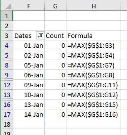
Figure 1.
2023-04-08 10:42:48
Allen
James, the approach using the MAX function is an alternative to using the SUBTOTAL function. And, yes, the formula (as I point out) goes into the column where you want the sequential count -- everything happens in column G in this example AFTER applying the filter.
-Allen
2023-04-08 10:21:51
J. Woolley
Here is something interesting about SUBTOTAL(Function_Num,...):
Function_Num 1-11 includes manually-hidden rows and 101-111 excludes them, but filtered-out cells are ALWAYS excluded.
2023-04-08 10:14:47
J. Woolley
@Allen
I don't understand. Did you mean that the MAX function in column G applies when the SUBTOTAL function is used in column F? If so, the MAX function in column G should be =MAX(F$1:F3), not =MAX($G$1:G3).
Also, in NumberVisibleRows2 you have mixed columns 8 and 7.
Got a version of Excel that uses the ribbon interface (Excel 2007 or later)? This site is for you! If you use an earlier version of Excel, visit our ExcelTips site focusing on the menu interface.
FREE SERVICE: Get tips like this every week in ExcelTips, a free productivity newsletter. Enter your address and click "Subscribe."
Copyright © 2026 Sharon Parq Associates, Inc.
Comments