Please Note: This article is written for users of the following Microsoft Excel versions: 2007, 2010, 2013, 2016, 2019, 2021, and Excel in Microsoft 365. If you are using an earlier version (Excel 2003 or earlier), this tip may not work for you. For a version of this tip written specifically for earlier versions of Excel, click here: Formatted Dates Appear Differently on Different Systems.
Written by Allen Wyatt (last updated November 16, 2024)
This tip applies to Excel 2007, 2010, 2013, 2016, 2019, 2021, and Excel in Microsoft 365
Edward has noticed a problem with formatted dates on different machines. Many times, he will create a workbook on one computer but use a different computer to print the report for inclusion in a mailing. Even though he has the cells formatted one way when he creates the report (i.e., the date is mm/dd/yy), when he opens the workbook on the second computer the date will appear differently (mm/dd/yyyy). This causes problems with the appearance of the final printed report as the cell data is then truncated.
Actually, the answer to this problem is similar to the discussion in the previous tip. The problem occurs because of differences in the way that system dates are set up on the two machines. On one machine the system date is set up in Windows to display using two digits for the year, while the other is set up to display using four.
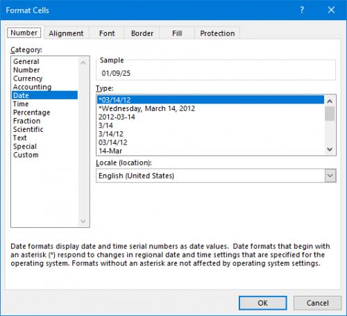
How does this affect Excel? Some of the date formats in Excel automatically use the system date format used by Windows. When you display the Number tab of the Format Cells dialog box you know that Excel provides a number of different date formats you can select. Note that some of the formats have an asterisk in front of them. These represent the "system date" formats. If you select one of these, it means that Excel uses the corresponding system date format to display the information in the cell. If you move the workbook to a different system and the formats used for system dates are different, then the dates will display differently in those cells.
The solution is to either change the system date formats to be the same on both systems (done in Windows, in the Regional Settings applet of the Control Panel), or simply pick a different date format in Excel. You'll want to pick one that doesn't have an asterisk in front of it or define your own custom date format. You should then have no problem with different displays of the dates on the different systems.
ExcelTips is your source for cost-effective Microsoft Excel training. This tip (9513) applies to Microsoft Excel 2007, 2010, 2013, 2016, 2019, 2021, and Excel in Microsoft 365. You can find a version of this tip for the older menu interface of Excel here: Formatted Dates Appear Differently on Different Systems.

Excel Smarts for Beginners! Featuring the friendly and trusted For Dummies style, this popular guide shows beginners how to get up and running with Excel while also helping more experienced users get comfortable with the newest features. Check out Excel 2013 For Dummies today!
Applying different formatting to the text within a cell can seem a bit confusing. This is certainly the case when it ...
Discover MoreWant to copy formatting from one cell and paste it into another cell? It's easy to do if you use the Paste Special ...
Discover MoreExcel allows you to adjust not only the horizontal alignment of values in a cell, but also the vertical alignment. This ...
Discover MoreFREE SERVICE: Get tips like this every week in ExcelTips, a free productivity newsletter. Enter your address and click "Subscribe."
2025-01-10 12:24:10
J. Woolley
@dave
My previous comment was incomplete. The answer to your question is given by the explanation at the bottom of the Format Cells dialog in Figure 1 below. If you want a format that does not "respond to changes in regional date and time settings" then pick a Date format that does not "begin with an asterisk" or specify a Custom format like d-mmm-yyyy or dd-mm-yyyy or dd/mmm/yyyy or dd_mmm_yyyy or dd-mmm-yy etc.
2025-01-09 16:34:17
J. Woolley
@dave
I assume you refer to the short date format specified in Windows Settings > Time & Language > Date & Time > Date, Time & Regional Formatting. When a date is displayed in a worksheet cell, you can change the cell's format by pressing Ctrl+1 or expanding Home > Number (Alt+H+FM) to show the Format Cells dialog, then pick a Date format or specify a Custom format (see Figure 1 below)

Figure 1.
2025-01-08 04:19:40
dave
Hi Allen,
I have a problem where I define a custom short date format in a sheet of dd-mmm-yyyy (UK style, e.g. 12-Jan-2025) which on a different systems gets seen as a long date format, i.e. 12-January-2025. It's not a problem with the year format, but the month. Is there a way to somehow 'embed' the format in the sheet?
Got a version of Excel that uses the ribbon interface (Excel 2007 or later)? This site is for you! If you use an earlier version of Excel, visit our ExcelTips site focusing on the menu interface.
FREE SERVICE: Get tips like this every week in ExcelTips, a free productivity newsletter. Enter your address and click "Subscribe."
Copyright © 2025 Sharon Parq Associates, Inc.
Comments