Filtering for Purchases within a Given Month

Anand has a worksheet that contains sales information consisting of customer names (column A) and purchase date (column B). He needs to filter the list so that he can see customers who purchased exactly X times within a given calendar month, where X is a value such as 1, 2, etc. He wonders if there is a way to do this using the built-in filtering or is another approach better.

There are actually several different ways you can approach this problem. Excel provides a number of different tools that could be used to derive a result, but I'll only focus on a couple of them. Both approaches require helper columns to use in your filtering.

The first approach uses just a single helper column. Assuming your data begins in row 2 and occupies no more than 99 rows, enter the following in cell C2:

=COUNTIFS($A$2:$A$100,A2,$B$2:$B$100,">="&
DATE(YEAR(B2),MONTH(B2),1),$B$2:$B$100,"<"&
DATE(YEAR(B2),MONTH(B2)+1,1))

This is a single formula; it returns a count of how many purchases the person in column A made within the month indicated by the date in column B. Copy the formula down as many rows as necessary for your data. With a cell in your data selected, display the Data tab of the ribbon and click the Filter tool in the Sort & Filter group. Excel displays the filter controls at the top of each column in your data.

Click the control at the top of the Date column to display the filtering palette, then pick the month you want to target. (In the years area at the bottom of the palette, clear the Select All check box, then select a year, and finally a month.) Click the control at the top of the helper column to pick how many sales you want in the filtered list. (See Figure 1.)

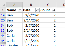
Figure 1. Your filtered data.

Note that the result shows multiple occurrences of each name for the target month. Thus, if you choose to display those that have purchased 3 times in a given month, you'll see 3 rows for any given name in the target month.

This is OK for a relatively low X rate for a month. However, if you want to see those who have purchased 50 times in a month, it quickly becomes unwieldy. Instead, you need a way to limit to a single instance of a given name within the filtered list.

This brings us to a solution that requires two helper columns, which I'll call Count and Tally. If your first cell in the Count column is C4, enter this into that cell:

=IF(EOMONTH(B4,0)<>EOMONTH($B$1,0),0,IF(A4=A3,C3+1,1))

Copy this formula down as far as necessary for your data. It returns a value of 0 unless the month and year is a match to the month and year in cell B1. (The date in cell B1 should be within your target month. It can be any date within that month.) If the month and year are a match, then the count increments for each sale for the same customer within that month.

If the first cell of the Tally column is cell D4, then place this formula in that cell:

=IF(C4>=C5,C4,0)

Copy this formula down the column, as well. The formula retains only the highest value from the Count column for any customer, setting all other values to 0.

Now, with any cell in your data selected, display the Data tab of the ribbon and click the Filter tool. Excel displays the filter controls at the top of each column in your data. (See Figure 2.)

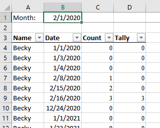
Figure 2. An example set of data.

You are now ready to get the desired information. Just sort the data first by column A (the Name column) and then by column B (the Date column). You can then use the drop-down filter control at the top of column D (the Tally column) to select how many sales you want for the desired month (which, remember, is specified in cell B1). If you specify that only the value 1 should be displayed, then you have the names of all the people who purchased just once in the month. If you select 2, then the displayed names are those who purchased twice, etc.

ExcelTips is your source for cost-effective Microsoft Excel training. This tip (9692) applies to Microsoft Excel 2007, 2010, 2013, 2016, 2019, and Excel in Microsoft 365.