Please Note: This article is written for users of the following Microsoft Excel versions: 2007, 2010, 2013, 2016, 2019, 2021, and Excel in Microsoft 365. If you are using an earlier version (Excel 2003 or earlier), this tip may not work for you. For a version of this tip written specifically for earlier versions of Excel, click here: Printing Comments.
Written by Allen Wyatt (last updated July 16, 2022)
This tip applies to Excel 2007, 2010, 2013, 2016, 2019, 2021, and Excel in Microsoft 365
Not only are comments handy when you are displaying your worksheet, but you can also print them out for a permanent record. Excel provides two ways to print comments. The first is as they are displayed on your worksheet. This method results in a graphic printout that shows comments over the top of your worksheet, as they appear when displayed on the monitor. Only those comments currently displayed on the screen are printed, however. If a comment is hidden, it is not printed at all.
The second method is to print the comments separately, at the end of the worksheet. The reference for a cell to which a comment is attached is printed first, followed by the comment itself. Thus, you might see the following on the printout:
   Cell: C4
Comment: Allen L. Wyatt:
         Prices last updated 10/12/22
Each comment is printed in this format, until all the comments are printed. This printing choice is a great way to provide a complete list of all the comments in a worksheet.
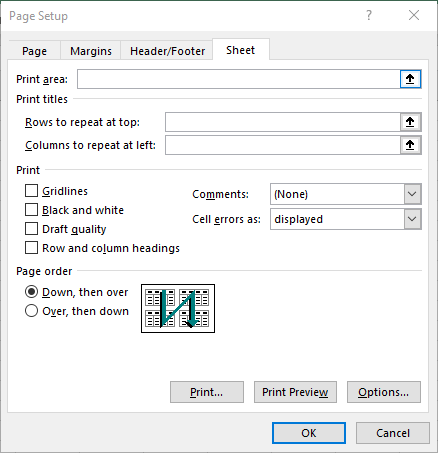
To control how comments are printed, follow these steps:

Figure 1. The Sheet tab of the Page Setup dialog box.
ExcelTips is your source for cost-effective Microsoft Excel training. This tip (10102) applies to Microsoft Excel 2007, 2010, 2013, 2016, 2019, 2021, and Excel in Microsoft 365. You can find a version of this tip for the older menu interface of Excel here: Printing Comments.

Excel Smarts for Beginners! Featuring the friendly and trusted For Dummies style, this popular guide shows beginners how to get up and running with Excel while also helping more experienced users get comfortable with the newest features. Check out Excel 2019 For Dummies today!
Pasting the contents of a single cell into a comment is rather easy. Pasting the contents of a range of cells is a ...
Discover MoreExcel allows you to use a picture as a background on a cell comment. This tip looks at how you can paste pictures into a ...
Discover MoreOne of the pieces of information that Excel can maintain relative to a workbook is a set of comments of your choice. ...
Discover MoreFREE SERVICE: Get tips like this every week in ExcelTips, a free productivity newsletter. Enter your address and click "Subscribe."
2022-07-16 15:37:20
J. Woolley
My Excel Toolbox includes the following dynamic array function:
=ListComments([AllSheets],[Threaded],[SkipHeader])
This function returns one row for each comment with the following columns: Worksheet, Cell, Author, Comment (text). It works with threaded and unthreaded Comments (Notes).
In older versions of Excel that do not support dynamic arrays, you can use ListComments with the SpillArray function like this:
=SpillArray(ListComments([AllSheets],[Threaded],[SkipHeader]))
SpillArray will determine and populate the spill range for its array expression argument, simulating a dynamic array.
See https://sites.google.com/view/MyExcelToolbox/
2022-07-16 09:08:37
Karen Prytula
Don't forget to check the 'Row and Column Headings' box too, so you can easily find the cell C4 in the printed document. C4 is pretty easy to find, but if the comment were in cell C234, you will have to start counting all the rows to find it otherwise.
Got a version of Excel that uses the ribbon interface (Excel 2007 or later)? This site is for you! If you use an earlier version of Excel, visit our ExcelTips site focusing on the menu interface.
FREE SERVICE: Get tips like this every week in ExcelTips, a free productivity newsletter. Enter your address and click "Subscribe."
Copyright © 2026 Sharon Parq Associates, Inc.
Comments