Formatting a PivotTable

You know that you can format cells in your worksheets by using the different tools on the various Ribbon tabs. Excel also allows you to format PivotTables using these same techniques. You should know, however, that the best way to format PivotTables is to use the AutoFormat feature. This is because whenever you manipulate the table or refresh the data, any explicit formatting you might have applied (using the Ribbon tabs) has a good chance of being eliminated by Excel. This limitation does not apply when you use the built-in AutoFormats.

To use the AutoFormat feature, select a cell in the PivotTable, and then use one of these techniques:

• Display the Home tab of the Ribbon and click Format as Table in the Styles group.
• Display the Design tab of the Ribbon (this tab is only visible when you select a cell in the PivotTable).

The differences between these two options are in how the available choices are accessed. If you choose the first option, you have a large number of table formats that can be applied to your PivotTable. If you choose the second option, then the same table formats are available, but it takes longer to scroll through them all.

It is also interesting that Excel allows you to define your own formats to be applied to PivotTables. This is very powerful, as it allows you to define and preserve just the formatting you want. Follow these steps:

1. Select a cell within your PivotTable.
2. Display the Home tab of the Ribbon and click Format as Table in the Styles group. Excel displays a whole host of options.
3. At the bottom of the available options click New PivotTable Style. Excel displays the New PivotTable Quick Style dialog box (Excel 2007 and Excel 2010) or the New PivotTable Style dialog box (later versions of Excel). (See Figure 1.)



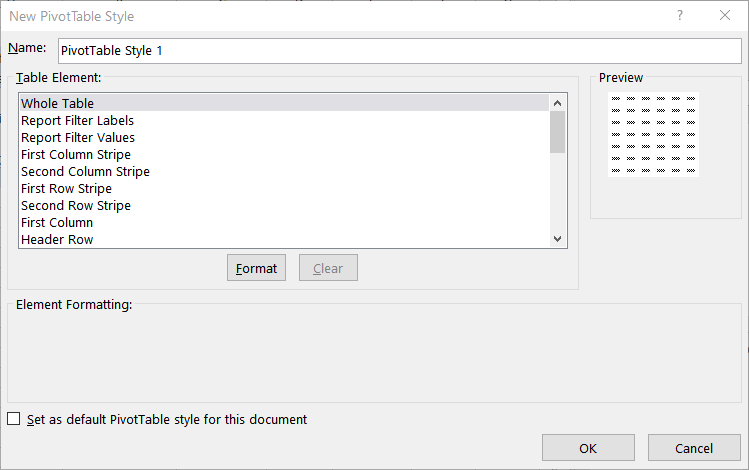
Figure 1. The New PivotTable Style dialog box.

Regardless of the name (which varies based on the version of Excel you are using), the dialog box allows you to independently select different parts of the PivotTable (called elements) and apply different formatting to them. You can get as detailed as you want and then save the style under the name specified at the top of the dialog box.

After a style is defined, you can apply it in the same way that you apply any other table style to your PivotTable.

ExcelTips is your source for cost-effective Microsoft Excel training. This tip (10283) applies to Microsoft Excel 2007, 2010, 2013, 2016, 2019, and Excel in Microsoft 365. You can find a version of this tip for the older menu interface of Excel here: Formatting a PivotTable.