By default, Excel places the worksheet tabs just below the worksheet and above the status bar. Benny wonders if it is possible to move the tabs to a different side of the worksheet. If he was able to move them to the left or right side, he believes he could see more of them at once.
There is no setting within Excel to indicate where tabs should appear, nor can you drag the tabs area to a different side of the program window. That being said, there are some things you can try.
First, you can use the Navigation pane. Display the View tab of the ribbon and click on the Navigation tool, and the pane appears at the right side of the screen. It defaults to showing all the worksheets in the workbook, but you can expand any worksheet in the pane to display elements of that worksheet.
Further, you can reposition the Navigation pane by hovering the mouse pointer over the top border, just to the right of the title "Navigation." The pointer turns into a four-headed arrow, at which point you can click and drag the Navigation pane to where you prefer it be located.
There are also third-party add-ins for Excel that can provide horizontal worksheet navigation lists. You can find such add-ins through an Internet search, or you can check out these:
If the entire purpose of wanting to move the worksheet tabs is to see more tabs on the screen at once, then there are other things you can try (while leaving the tabs at the bottom of the screen). For instance, you can resize or hide the horizontal scroll bar. You can resize it by clicking on the three dots at the left of the scroll bar and drag to the right. You can turn it off by following these steps:
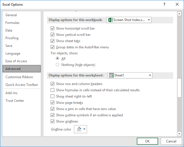
Figure 1. The Advanced options of the Excel Options dialog box.
To display even more worksheet tabs, consider renaming your worksheets with shorter names. Excel will adjust the size of the tabs according to the length of the worksheet names and the number of worksheets in the workbook. The shorter the names, the more tabs you can see.
Finally, notice that to the left of the worksheet tabs there is a < and a > character. Hover the mouse over these and you can see that you can use the arrows for navigation. Right-clicking on either arrow displays a list of worksheets in a dialog box, allowing you to easily jump to the one you want.
ExcelTips is your source for cost-effective Microsoft Excel training. This tip (10622) applies to Microsoft Excel 2007, 2010, 2013, 2016, 2019, 2021, 2024, and Excel in Microsoft 365.

Professional Development Guidance! Four world-class developers offer start-to-finish guidance for building powerful, robust, and secure applications with Excel. The authors show how to consistently make the right design decisions and make the most of Excel's powerful features. Check out Professional Excel Development today!
Need to know the name of the current worksheet? You can use the CELL function as the basis for finding this information ...
Discover MoreExcel makes it easy to change the color of a worksheet's tab. If you want that color change to be dynamic, one way to do ...
Discover MoreIf you spend a lot of time creating a worksheet, you might want to make multiple copies of that worksheet as a starting ...
Discover MoreFREE SERVICE: Get tips like this every week in ExcelTips, a free productivity newsletter. Enter your address and click "Subscribe."
2025-05-20 20:48:48
Bob
The MVP's out there could no doubt improve on the code below which is a fairly simple solution to gathering the tab names vertically.
Bob D.
Option Explicit
Option Base 1
Static Sub List_Tab_Names()
'' List only visible sheets
Dim i As Integer
Dim t As String
Dim MyCell
t = "List Tab Names"
Dim Status(-1 To 2) As String
Status(-1) = "Visible"
Status(0) = "Hidden"
Status(2) = "VeryHidden"
On Error GoTo Err_1:
With Application
.ScreenUpdating = False
End With
' Does TabNames Sheet Already Exist?
With ActiveWorkbook
If Evaluate("isref('" & "TabNames'!A1)") Then
GoTo Start_2:
Else
GoTo Start_1:
End If
End With
' If Not Create New Sheet
Start_1:
With ActiveWorkbook
.Sheets.Add Before:=Worksheets(1)
ActiveSheet.Name = "TabNames"
End With
' AND/OR Update new/existing sheet
Start_2:
Sheets("TabNames").Select
[A:A].Select
With Selection
.ClearContents
End With
[A5].Select
With Selection
For i = 1 To Worksheets.Count
If Status(Worksheets(i).Visible) <> Status(-1) Then GoTo Resume_1:
.Offset(i, 0) = Worksheets(i).Name
Resume_1:
Next i
End With
[A1].Select
With ActiveSheet
With .Range("A5:C200")
.Columns.AutoFit
.Sort key1:=ActiveCell, Header:=xlYes
End With
End With
[A6].Select
ActiveCell.CurrentRegion.Select
For Each MyCell In Selection
MyCell.Select
Selection.Hyperlinks.Add Anchor:=Selection, Address:="", SubAddress:=ActiveCell.Value & "!A1"
Next MyCell
' Window Dressing
[A1] = "Created - "
[A2].Value = Date
[A3].Value = Time
[A5].Value = "WB Tab Names:"
[A1:A5].Font.Bold = True
[A1:A5].Font.Color = vbBlack
Columns("A:A").AutoFit
Columns("A:A").HorizontalAlignment = xlCenter
Columns("B:B").Select
ActiveWindow.FreezePanes = True
Selection.Interior.ColorIndex = 15
[A1].Select
GoTo Endline:
Err_1:
MsgBox Error, 16, t
GoTo Endline:
Endline:
With Application
.ScreenUpdating = True
.CutCopyMode = False
End With
End Sub
2025-05-17 14:44:22
J. Woolley
To quickly move from sheet to sheet, use Ctrl+PageDown and Ctrl+PageUp keyboard shortcuts.
To toggle the horizontal scrollbar (and other properties of Excel's window), use My Excel Toolbox's WindowDressing macro (see Figure 1 below) ; you might find it more convenient than the File > Options procedure.
See https://sites.google.com/view/MyExcelToolbox
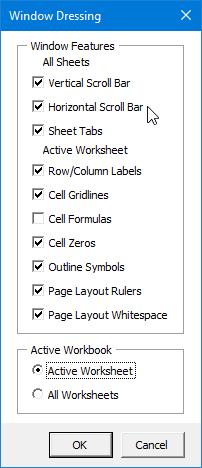
Figure 1.
Got a version of Excel that uses the ribbon interface (Excel 2007 or later)? This site is for you! If you use an earlier version of Excel, visit our ExcelTips site focusing on the menu interface.
FREE SERVICE: Get tips like this every week in ExcelTips, a free productivity newsletter. Enter your address and click "Subscribe."
Copyright © 2026 Sharon Parq Associates, Inc.
Comments