Retaining Formatting After a Paste Multiply

One of the really cool features of Excel is the many ways you can manipulate data using the Paste Special command. This command allows you to do all sorts of things to your data as you paste it into a worksheet. One such manipulation you can perform is to multiply data as you paste. For instance, you can multiply all the values being pasted by -1, thereby converting them into negative numbers. To do so, follow these steps:

1. Place the value -1 in an unused cell of your worksheet.
2. Select the value and press Ctrl+C. Excel copies the value (-1) to the Clipboard.
3. Select the range of cells that you want to multiply by -1.
4. Display the Home tab of the ribbon.
5. Click the down-arrow under the Paste tool, and then click Paste Special. Excel displays the Paste Special dialog box. (See Figure 1.)



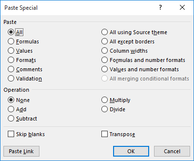
Figure 1. The Paste Special dialog box.

6. Click on the Multiply radio button.
7. Click on OK.

At this point Excel multiplies the values in the selected cells by the value in the Clipboard. Unfortunately, if the cells in the selected range had special formatting, the formatting is also now gone, and the format of the cells is set to be the same as the cell you selected in step 2.

To make sure that the formatting of the target cells is not changed while doing the Paste Special, there is one other option you need to select in the Paste Special dialog box—Values. In other words, you would still select Multiply (as in step 6), but you would also select Values before clicking on OK.

With the Values radio button selected, Excel only operates on the values in the cells, and leaves the formatting of the target range unchanged.

ExcelTips is your source for cost-effective Microsoft Excel training. This tip (10813) applies to Microsoft Excel 2007, 2010, 2013, 2016, 2019, and Excel in Microsoft 365. You can find a version of this tip for the older menu interface of Excel here: Retaining Formatting After a Paste Multiply.