Please Note: This article is written for users of the following Microsoft Excel versions: 2007, 2010, 2013, 2016, 2019, 2021, and Excel in Microsoft 365. If you are using an earlier version (Excel 2003 or earlier), this tip may not work for you. For a version of this tip written specifically for earlier versions of Excel, click here: Filtering for Comments.
Written by Allen Wyatt (last updated August 5, 2023)
This tip applies to Excel 2007, 2010, 2013, 2016, 2019, 2021, and Excel in Microsoft 365
Robert has a worksheet that has comments included in various places. (These are the traditional comments, now called notes by Microsoft.) He wonders if it is possible to filter the rows in a data table so that only those rows that include comments in a particular column are displayed.
The filtering capabilities of Excel don't provide a way that you can automatically check for the presence of comments/notes, but there are a couple of ways you can approach a solution. One possible solution is to follow these general steps:
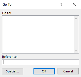
Figure 1. The Go To dialog box.
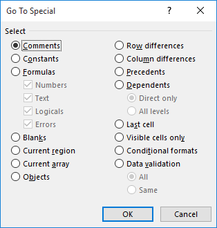
Figure 2. The Go To Special dialog box.
If you prefer, you can create a user-defined function that will let you know if a particular cell has a comment associated with it. The following is a simple way to make such a determination:
Function CellHasComment(c As Range)
    Application.Volatile True
    CellHasComment = Not c.Comment Is Nothing
End Function
Now you can use a formula such as the following within a worksheet:
=CellHasComment(B2)
When the formula is executed, it returns either True or False, depending on whether cell B2 has a comment or not. You can then use Excel's filtering capabilities to display only those rows that have a True returned by the formula.
Note:
ExcelTips is your source for cost-effective Microsoft Excel training. This tip (11232) applies to Microsoft Excel 2007, 2010, 2013, 2016, 2019, 2021, and Excel in Microsoft 365. You can find a version of this tip for the older menu interface of Excel here: Filtering for Comments.

Program Successfully in Excel! This guide will provide you with all the information you need to automate any task in Excel and save time and effort. Learn how to extend Excel's functionality with VBA to create solutions not possible with the standard features. Includes latest information for Excel 2024 and Microsoft 365. Check out Mastering Excel VBA Programming today!
If you frequently add comments to cells in a worksheet, Excel provides a variety of tools you can use to manage those ...
Discover MorePasting the contents of a single cell into a comment is rather easy. Pasting the contents of a range of cells is a ...
Discover MoreWhen you print your worksheet, you may want Excel to include your comments or notes as they appear on the screen. Here's ...
Discover MoreFREE SERVICE: Get tips like this every week in ExcelTips, a free productivity newsletter. Enter your address and click "Subscribe."
2023-08-11 16:15:42
J. Woolley
My Excel Toolbox includes the following dynamic array function to list a worksheet's auto filters (Data > Filter):
=ListAutoFilters([Target],[SkipHeader])
It returns three rows (filter range, head cell's value, filter criteria) for Target's worksheet with one column for each filter plus an optional header column. Target can be a cell or range on any worksheet in an open workbook; if omitted, the formula's cell is assumed. If SkipHeader is FALSE (default), a header will be returned in the first column; otherwise, there will be no header column. You can swap rows and columns like this:
=TRANSPOSE(ListAutoFilters(...))
My Excel Toolbox's SpillArray function (described in UseSpillArray.pdf) simulates a dynamic array in older versions of Excel.
See https://sites.google.com/view/MyExcelToolbox
2023-08-10 13:15:55
J. Woolley
Updating a suggestion by Willy Vanhaelen, you can define a conditional format rule to color cells that have a comment, then apply a filter based on cell color.
The following procedure assumes use of the HasComment function described in my previous comment below. If HasComment is located in another workbook or an Excel add-in file like MyToolbox.xlam, it cannot be directly referenced in a conditional format rule; therefore, a defined name (named range) is used instead:
1. Click Formulas > Defined Names > Define Name... and specify
Name: CommentCell
Scope: Workbook
Comment: TRUE if this cell has a comment
Refers to: =HasComment()
2. Select the range of cells with comments you want to filter.
3. Click Home > Styles > Conditional Formatting > New Rule... and specify
Rule type: Use a formula...
Where this formula is True: =CommentCell
Format: Fill (specify a color)
Then each cell with a comment in the conditional format range will have the specified fill color. Now you can apply a filter based on that color to isolate table cells that have a comment.
Note: To initiate Filter by Color, there must be no blank cells below the filter header down to and including the colored comment cells.
2023-08-05 14:46:00
J. Woolley
The Tip addresses "rows that include comments in a particular column" and only "traditional comments" are considered.
My Excel Toolbox includes the following function returning TRUE if any cell in Target includes a comment:
=HasComment([Target],[Threaded])
Target is the range of cells to consider; default is the formula's cell.
If Threaded is TRUE, only new threaded Comments will be considered; default is FALSE for traditional unthreaded comments (Notes). To consider both for several columns in a row (like columns A:F in row 2):
=OR(HasComment(A2:F2,TRUE),HasComment(A2:F2))
If this formula is copied down several rows, it will return TRUE if any cell in the first 6 columns of each row has either type of comment.
See https://sites.google.com/view/MyExcelToolbox/
Got a version of Excel that uses the ribbon interface (Excel 2007 or later)? This site is for you! If you use an earlier version of Excel, visit our ExcelTips site focusing on the menu interface.
FREE SERVICE: Get tips like this every week in ExcelTips, a free productivity newsletter. Enter your address and click "Subscribe."
Copyright © 2025 Sharon Parq Associates, Inc.
 Please Note:
This article is written for users of the following Microsoft Excel versions: 2007, 2010, 2013, 2016, 2019, 2021, and Excel in Microsoft 365. If you are using an earlier version (Excel 2003 or earlier), this tip may not work for you. For a version of this tip written specifically for earlier versions of Excel, click here:
Please Note:
This article is written for users of the following Microsoft Excel versions: 2007, 2010, 2013, 2016, 2019, 2021, and Excel in Microsoft 365. If you are using an earlier version (Excel 2003 or earlier), this tip may not work for you. For a version of this tip written specifically for earlier versions of Excel, click here:
Comments