Please Note: This article is written for users of the following Microsoft Excel versions: 2007, 2010, 2013, 2016, 2019, 2021, 2024, and Excel in Microsoft 365. If you are using an earlier version (Excel 2003 or earlier), this tip may not work for you. For a version of this tip written specifically for earlier versions of Excel, click here: Last Non-Zero Value in a Row.
Brian has a row of numbers with 240 cells. In this row, the numbers are steadily declining and will eventually, at some point in those 240 cells, become 0. The zeroes will continue to fill the remaining cells in the row. Brian needs to write an equation that will return the last non-zero value in the row.
There are a variety of ways that the desired value can be returned. (Doesn't that always seem to be the case with Excel? You can come up with lots of ways to get a result.) In general, you could use a regular formula or an array formula.
If you want to use a regular formula, here's one you can try:
=OFFSET(A6,0,(COUNT(A6:IF6)-COUNTIF(A6:IF6,0))-1)
The COUNTIF function counts the number of zero values and the COUNT function determines the number of cells in the range. Subtracting one from the other and adjusting by 1 gives the OFFSET value into the "array" of cells where the last non-zero value lies. This formula assumes that the values begin in column A; if they begin in a different column then you'll need to adjust the value provided by the COUNT/COUNTIF portion of the formula to represent the offset from the first column.
Here's a shorter variation of the formula, based on doing an offset from the right side of the range rather than the left side:
=OFFSET(IF6,0,-COUNTIF(A6:IF6,0))
In this instance it is important that IF6 be the actual right end of the range. The formula works by counting the number of zero values in the range (all at the right side of the range) and then computing the cell address of the last cell (IF6) minus the number of zeros.
Here is a version that uses the INDEX function, instead:
=INDEX(A6:IF6,,MATCH(0,A6:IF6,0)-1)
This version is even shorter, using the LOOKUP function:
=LOOKUP(1,1/(6:6>0),6:6)
If you are using Excel 2021 or Excel in Microsoft 365, you can use the XLOOKUP version of the formula:
=XLOOKUP(TRUE,6:6>0,6:6,0,,-1)
Array formulas can also be used. (In versions of Excel before Excel 2021, array formulas are entered by pressing Ctrl+Shift+Enter. In later versions, no special entry steps are required.) This one uses the INDIRECT function:
=INDIRECT("R6C" & MAX((A6:IF6>0)*COLUMN(A6:IF6)),FALSE)
This array formula uses an interesting implementation of the LOOKUP function to find the correct result:
=LOOKUP(9.99999999999999E+307,IF(A6:IF6<>0,A6:IF6))
Here's another array formula that can be used, this time using the OFFSET function to find the last non-zero value in row 6:
=OFFSET(A6,0,MIN(IF(6:6=0,COLUMN(6:6),300))-2)
Here's an even shorter variation:
=MIN(IF(A6:IF6>0,A6:IF6))
All of these formulas presented so far depend on the fact that the numbers in the row actually do decline—they go from whatever the beginning number is and steadily go toward zero. If the numbers don't decline, then you can use a different type of array formula to determine the last non-zero value in the row:
=INDEX(6:6,MAX(IF(A6:IF6<>0,COLUMN(A6:IF6))))
The formula first determines the maximum column in the row (in this case row 6) that has a value not equal to zero, then it uses the INDEX function to get the value from that column in that row.
As you can tell, there are quite a few ways to find the last non-zero value in a row. Pick the one that strikes your fancy; there is no right or wrong in this instance.
ExcelTips is your source for cost-effective Microsoft Excel training. This tip (11250) applies to Microsoft Excel 2007, 2010, 2013, 2016, 2019, 2021, 2024, and Excel in Microsoft 365. You can find a version of this tip for the older menu interface of Excel here: Last Non-Zero Value in a Row.

Create Custom Apps with VBA! Discover how to extend the capabilities of Office 365 applications with VBA programming. Written in clear terms and understandable language, the book includes systematic tutorials and contains both intermediate and advanced content for experienced VB developers. Designed to be comprehensive, the book addresses not just one Office application, but the entire Office suite. Check out Mastering VBA for Microsoft Office 365 today!
Need to figure out if a value is outside of some arbitrary limit related to a different value? There are a number of ways ...
Discover MoreOne of the staples of high school algebra classes is the quadratic equation. If you need to solve such equations in ...
Discover MoreWhen analyzing data, you may have a need to calculate a sum based on just part of a particular cell. This tip examines ...
Discover MoreFREE SERVICE: Get tips like this every week in ExcelTips, a free productivity newsletter. Enter your address and click "Subscribe."
2022-03-28 08:08:50
Evelina
Thank You, @J. Woolley!
The first formula worked like charm.
2022-03-25 15:56:39
J. Woolley
@Evelina
If you have the latest version of Excel with support for the LET function, this formula will work for your example (which uses semicolon instead of comma within a formula):
=LET(x;FREQUENCY(IF(D10:AP10>0;COLUMN(D10:AP10));IF(D10:AP10=0;COLUMN(D10:AP10)));INDEX(x;ROWS(x)))
If you can't use the LET function, this formula also works (assuming sales never have negative values):
=INDEX(FREQUENCY(IF(D10:AP10>0;COLUMN(D10:AP10));IF(D10:AP10=0;COLUMN(D10:AP10)));(COLUMNS(D10:AP10)-COUNTIF(D10:AP10;">0")+1))
Notice FREQUENCY returns a vertical array and you want the last row of that array.
2022-03-25 02:36:10
Evelina
Hello,
I have a question about counting the number of last non-zero months of sales in a row (until the first month of zero sales).
For example - I have a row with following monthly sales 1, 1, 1, 1, 1, 1, 0, 1, 1, 1 (1 for a month with sales, 0 - no sales).
The needed answer for this example should be 3 months (counting the LAST 3 months with sales).
I have been using a formula like this (D10:AP10 the first row):
=MAX(FREQUENCY(IF(D10:AP10>0;COLUMN(D10:AP10));IF(D10:AP10=0;COLUMN(D10:AP10))))
But using this formula the answer to my example would be 5, counting the max of consecutive months of sales, ignoring the condition of LAST months of sales.
Any help would be appreciated!
2021-01-23 01:58:43
TS
I just wanted to say thank you! I was on the verge of giving up but I'm glad I found this clear article! The first formula you suggested worked perfectly for what I was working on in G Sheets.
2019-02-13 04:56:24
SoniboiTM
Oh! This works.
=OFFSET(AC181,0,MATCH(MAX(AC181:XFD181)+1,AC181:XFD181,1)-1)
---------------------------------------------------------
My previous comment:
Hi, guyz!
Tried some formulas, including this one:
=LOOKUP(1,1/(6:6>0),6:6)
But got inaccurate report if the last value = 0.00.
Any solution?
Thanks.
2019-02-13 04:44:54
SoniboiTM
Hi, guyz!
Tried some formulas, including this one:
=LOOKUP(1,1/(6:6>0),6:6)
But got inaccurate report if the last value = 0.00.
Any solution?
Thanks.
2019-01-30 03:48:38
George,
The following "formula" versions should work to find you the, last non empty, 2nd & 3rd to last empty row number. You will have to change the column references in the Indirect references by hand if you copy the formulas to different columns as they are text & will not adjust automatically.
=MATCH(9.99^308,B:B,1)
=MATCH(9.99^308,INDIRECT("B1:B"&(MATCH(9.99^308,B:B,1)-1)),1)
=MATCH(9.99^308,INDIRECT("B1:B"&MATCH(9.99^308,INDIRECT("B1:B"&(MATCH(9.99^308,B:B,1)-1)),1)-1),1)
(see Figure 1 below)
hope this helps
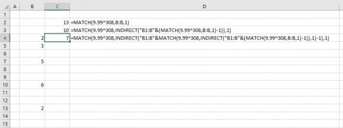
Figure 1. example
2019-01-29 04:41:00
I've been searching around for formulas (no VBA) to give me the last non-empty cell in a column, then another for the 2nd to last non-empty cell in a column, then third to last non-empty cell in a column, etc.......... to place in separate cells. I've had no luck with the 2nd to last and so forth. Can you help me with this? I would appreciate the help.
2018-12-06 20:27:20
Peter Atherton
Igor
Ive gone the macro way. With the Sub place the cursor in Column A on the same row as the data
Sub CountBlankAreas1()
Dim r As Long, lastColumn As Integer
Dim counter As Integer, i As Integer
r = ActiveCell.Row
lastColumn = Cells(r, Columns.Count).End(xlToLeft).Column
For i = lastColumn To 2 Step -1
If IsEmpty(Cells(r, i)) And Not IsEmpty(Cells(r, i - 1)) Then
counter = counter + 1
End If
Next
Cells(r, 1) = counter
End Sub
With the Function place it on the same row as the data say A1 and type +CountBlankAreas(A2)
Function COUNTBLANKAREAS(ByVal ref As Range)
Dim r As Long, lastColumn As Integer
Dim counter As Integer, i As Integer
Dim rng As Range
Application.Volatile
r = ref.Row
lastColumn = Cells(r, Columns.Count).End(xlToLeft).Column
Set rng = Range(Cells(r, 2), Cells(r, lastColumn))
For i = 1 To rng.Columns.Count - 1
If IsEmpty(rng(i)) And Not IsEmpty(rng(i + 1)) Then
counter = counter + 1
End If
Next
COUNTBLANKAREAS = counter
End Function
The function will recalculate when change, the Sub will not. But you can call it from a Worksheet_Change macro. Just make sure that the correct cell is activated first.
HTH
2018-12-06 11:41:14
Jed,
Not entirely sure I understand your question, I think you are trying to sum a range of undetermined location & size. If so the following should work
=SUM(OFFSET(G1,MATCH(COUNT(ISBLANK(G:G)),G:G,1)-1,,MATCH(9.99^308,G:G,1)))
This will find the first cell in a column that's not blank -1 that sets the first argument of offset, then finds the last cell with an entry, this sets the height of the offset range. The sum wrapped around the offset function sums the whole offset range. If you don't want to sum the range you can change the sum function to count or average or whatever you're trying to achieve.
2018-12-06 04:43:52
Hi Igor Ungurean
I expect this can be done in lots of ways, I did it in a combination of formulas, ( which , of course , you could combine to one formula )
Example
In A1 to F1 I have
1 , blank , 1 , 1 , blank , blank
The down column G , I have the following formulas as shown in the screenshot.
In words what I am doing
G1 – replace all blanks with x and concatenate all cell values in the range A1:F1
G2 – count the number of 1s in the range A1:F1
G3 – replace the last “1” in G1 with a W
G4 - Find the position along of that W
G5 – take just the left of the concatenated string up to where the W is
G6 – replace all the “1”’s in the string in G5 with nothing
G7 – effectively I count the number of x’s in G6 , which is effectively all the blanks up to the last “1” in the original range
The only problem you may have is with the first formula being too long.
Alan Elston
Formulas G1:G7
=IF(A1=1,1,"x") & IF(B1=1,1,"x") & IF(C1=1,1,"x") & IF(D1=1,1,"x") & IF(E1=1,1,"x") & IF(F1=1,1,"x")
=COUNTIF(A1:F1,1)
=SUBSTITUTE(G1,1,"W",G2)
=SEARCH("W",G3)
=LEFT(G1,G4)
=SUBSTITUTE(G5,1,"")
=LEN(G6)
(see Figure 1 below)
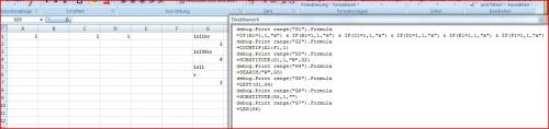
Figure 1.
2018-12-06 03:38:01
Steve Jez
Igor,
Sorry, posted too soon.
This assumes the formula will be in Col A and counting columns B > the last column with data. If you need a different range then change "B". It also assumes that the data contained in the cells is only 1 (less than 99 in the match function)
2018-12-06 03:30:54
Steve Jez
Igor,
I think the following, whilst slightly unwieldy, will do what you are trying to do.
=COUNTBLANK(INDIRECT("B"&ROW()&":"&ADDRESS(ROW(),MATCH(99,INDIRECT(ROW()&":"&ROW()),1))))
Hope this helps.
2018-12-05 15:14:49
Hi everyone, I'm still not able to figure out this:
There is a row with 300 cells, the only values in these cells are "1". What I need is to count all blank spaces among values, and don't count blanks after the last value in the row.
Ex:
1 , 1 , 1, blank , 1 , 1 , blank , blank , 1 , 1 , 1 , 1 ,blank , blank , blank , blank , blank , blank , blank , blank.
The result should be 3.
I try to implement this into COUNTBLANK, but still not able to make it count only blanks among values.
2018-11-17 19:17:10
Jed
I am trying to find the first blank cell in a column, where the colum beginning and end points are variable. (e.g row 5 to row 12) and the next may be (row 235 to row 720). These beginning and end points are functions of other calculations in the spreadsheet. I have tried combinations of Offset, Match, Row and Index functions. I am trying not to use VBA. Any thoughts?
2018-08-11 12:30:47
Peter Atherton
Amy
Try
=INDIRECT(ADDRESS(6,COUNTA(6:6)-1))
for row 6, providing no blanks in any column
2018-08-10 08:43:03
amy
How can I find the second to last value in a row?
2018-05-15 03:21:59
Sonny Cullo
Thanks.
This works fine: =LOOKUP(1,1/(6:6>0),6:6)
2018-03-02 06:17:58
Steve Jez
Some.Dude,
If you enter some sample data in a sheet & then use "Evaluate Formula" from the Formulas Ribbon Tab it might help. You will have to put the formula as written in any row other than row 6 or you will get a circular reference.
When the formula evaluates you will see;
(6:6>0) you see Trues or Falses then 1 or 0 for the content of row 6
(1/1 or 0) you see 1 or #Div/0! - the last cell which is not blank or zero will evaluate to 1
(1,(1 or #Div/0!) lookup is now trying to find 1 in an array of 1's & #Div/0! & it tries to find the last one (it's the way it is programmed), so when it finds the last 1 it returns the cell value of row 6
You don't have to use whole row references, I have used it to report the latest revision in col C in the format =lookup(1,1/D6:IV6>0),D6:IV6) the only caveat is that the 2 ranges must be the same size.
It's not massively intuitive, but I hope this helps.
2018-03-01 10:59:12
Some.Dude
Re: Last Non-Zero Value in a Row
=LOOKUP(1,1/(6:6>0),6:6)
Can anyone please help me understand how/why this formula works?
2018-02-20 12:09:55
Peter Atherton
GSR
Try the following, works from the last cell in the range, in your case M17
=COUNTIF(OFFSET($M17,0,-4,,5),"<"&0.98)
2018-02-19 12:32:50
GSR
I have a 2 rows in excel table.- 1st row is for Month and 2nd row is for score. The table is dynamic that a new month is added after every month. I need a formula which counts the score less than 98% from last 5 cells. I am trying something like-
=OFFSET($D$17,0,1,COUNTIF(D17:M17, "<0.98"),-5)
but this ain't working. Can someone help me.
e.g
if I have scores of 95%, 97%, 96%, 95%, 95%, 98%, 98%, 97%, 99%
The formula should show me the outcome as 2 as 2 values out of last 5 values have score less than 98%
2017-11-07 10:44:42
The first OFFSET formula worked great for me. Thanks! The formula will also return the second to last non-zero value in the row by changing the 1 at the end of the formula to 2, changing it to 3 the third to last etc.
Got a version of Excel that uses the ribbon interface (Excel 2007 or later)? This site is for you! If you use an earlier version of Excel, visit our ExcelTips site focusing on the menu interface.
FREE SERVICE: Get tips like this every week in ExcelTips, a free productivity newsletter. Enter your address and click "Subscribe."
Copyright © 2026 Sharon Parq Associates, Inc.
 Please Note:
This article is written for users of the following Microsoft Excel versions: 2007, 2010, 2013, 2016, 2019, 2021, 2024, and Excel in Microsoft 365. If you are using an earlier version (Excel 2003 or earlier), this tip may not work for you. For a version of this tip written specifically for earlier versions of Excel, click here:
Please Note:
This article is written for users of the following Microsoft Excel versions: 2007, 2010, 2013, 2016, 2019, 2021, 2024, and Excel in Microsoft 365. If you are using an earlier version (Excel 2003 or earlier), this tip may not work for you. For a version of this tip written specifically for earlier versions of Excel, click here:
Comments