How Many Times Does Each Name Appear in a List?

Richard used the UNIQUE function on a table of around 900 rows of different firms. The function identified the 600 or so unique firm names. He wonders if there is a way to figure out how many times each of the unique firms appears in the table, perhaps by combining UNIQUE with a different function.

There are actually a couple of different ways you can derive the information you want. Before providing solutions, however, it is best to lay out some parameters. Let's say that your firm names are in column A, with a column header in cell A1. This means your data is in the range A2:A901, for a total of 900 rows. Your unique list (using the UNIQUE function) is placed in cell C2, as follows:

=UNIQUE(A2:A901)

This provides you with 600 unique firm names, spilled into the range C2:C601. You could, if desired, sort the list of unique names by simply wrapping the formula in cell C2:

=SORT(UNIQUE(A2:A901))

You still end up with the 600 unique names, but they are now in alphabetical order. You can determine how many times each of the unique names appears in your original list by placing a formula into cell D2, right next to your UNIQUE formula:

=COUNTIF($A$2:A$901,C2)

Copy this down to the rest of the rows (D3:D601), and you'll have your counts.

It is obvious that Richard is using the version of Excel provided with Microsoft 365, otherwise he wouldn't be able to use the UNIQUE function. Because he is using this version, he could modify these last steps just a bit. With nothing in column D, add this variation of the formula into cell D2:

=COUNTIF($A$2:A$901,C2#)

Notice the addition of the hash mark at the end. Making this single-character change causes the results of the formula to spill down, as many cells as necessary, to provide results for the cells in column C. In other words, no copying of the formula to D3:D601 is necessary, and Richard has the counts he wants.

What if you are not using a newer version of Excel that supports the spillable functions like UNIQUE? If so, the traditional way of getting the unique values and counts is to use Excel's advanced filtering capabilities. Here are a couple of past tips I've written that describe how to use this capability:

https://tips.net/T7562
https://tips.net/T8732

Use the advanced filtering to pull the unique firm names (instead of using the UNIQUE function), and then you can use the COUNTIF formula (without the hash mark) to derive the number of instances that each unique firm name appears in your original list.

Finally, regardless of the version of Excel you are using, you could get your unique firm names and counts by creating a very simple PivotTable.

1. Select a cell within your data table.
2. Make sure the Insert tab of the ribbon is displayed.
3. In the Tables group, click the PivotTable tool.
4. Excel displays the Create PivotTable dialog box. (See Figure 1.)



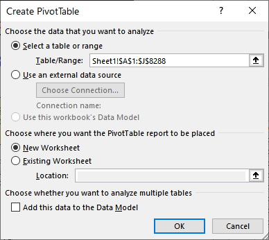
Figure 1. The Create PivotTable dialog box.

5. In the Range box, make sure your entire data table is selected, then click on OK. Excel creates an empty PivotTable worksheet.
6. Drag the Name field from the field list to the Rows area.
7. Drag the Name field from the field list to the Values area.

That's it; your PivotTable is complete. Because you placed the Name field in both the Rows and Values areas, you end up with a sorted list of unique firm names and a count of how many times each name appears in your original data.

ExcelTips is your source for cost-effective Microsoft Excel training. This tip (12856) applies to Microsoft Excel 2007, 2010, 2013, 2016, 2019, Excel in Microsoft 365, and 2021.