Please Note: This article is written for users of the following Microsoft Excel versions: 2007, 2010, 2013, 2016, 2019, 2021, and Excel in Microsoft 365. If you are using an earlier version (Excel 2003 or earlier), this tip may not work for you. For a version of this tip written specifically for earlier versions of Excel, click here: Hiding Graphics when Filtering.
Written by Allen Wyatt (last updated September 14, 2024)
This tip applies to Excel 2007, 2010, 2013, 2016, 2019, 2021, and Excel in Microsoft 365
James has a worksheet that has graphics on top of cells that explain what is in the cells. The graphics sort with the cells just fine, but when he applies filters to the cells, the graphics bunch up at top of cells that are visible. James wonders if there is a way to have graphics hide when filtering data within cells.
The answer has to do with how you have the properties for the graphics set up. You need to make sure that the graphics are set to resize when the row height changes. Here's what you do if you are using Excel 2013 or a later version:
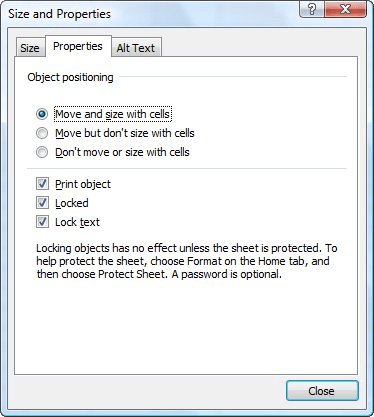
Figure 1. The Properties option of the Format Picture task pane.
If you are using Excel 2007 or Excel 2010, then the process is just a bit different because those versions don't use task panes. Follow these steps:
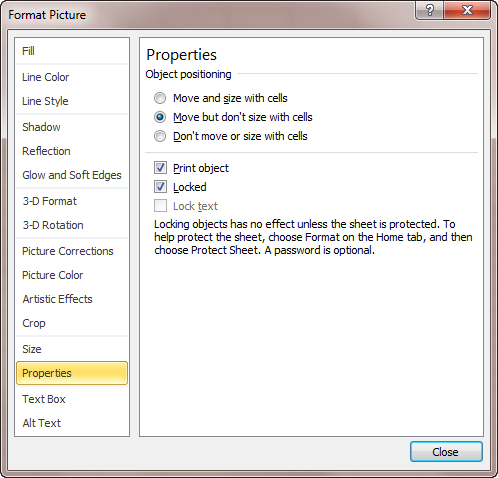
Figure 2. The Properties tab of the Size and Properties dialog box.
Regardless of your version of Excel, it is step 5 that does the trick. Since your graphics are sorting properly when you sort the worksheet, chances are good that you had the Move but Don't Size with Cells check box selected. This is what caused the graphics to bunch up—they couldn't resize when filtering hid the rows with which they were associated.
ExcelTips is your source for cost-effective Microsoft Excel training. This tip (11763) applies to Microsoft Excel 2007, 2010, 2013, 2016, 2019, 2021, and Excel in Microsoft 365. You can find a version of this tip for the older menu interface of Excel here: Hiding Graphics when Filtering.

Dive Deep into Macros! Make Excel do things you thought were impossible, discover techniques you won't find anywhere else, and create powerful automated reports. Bill Jelen and Tracy Syrstad help you instantly visualize information to make it actionable. You�ll find step-by-step instructions, real-world case studies, and 50 workbooks packed with examples and solutions. Check out Microsoft Excel 2019 VBA and Macros today!
Want to draw a few simple shapes or lines on your worksheet? It really is simple; here's how to do it.
Discover MoreExcel makes it rather easy to add shapes to your worksheets. If you add a lot of shapes, you quickly discover that it can ...
Discover MoreIf you have a group of merged cells into which you want a user to enter information, you may want some sort of ...
Discover MoreFREE SERVICE: Get tips like this every week in ExcelTips, a free productivity newsletter. Enter your address and click "Subscribe."
2024-09-16 10:35:39
J. Woolley
Excel graphics are called shapes. They can be grouped and/or linked to a formula, macro, or hyperlink. My Excel Toolbox includes the following dynamic array function to list information about a workbook's shapes:
=ListShapes([AllSheets], [SkipHeader], [IncludeText])
These 7 columns are returned for each shape: Range, Group, Type, Shape Name, Link Formula, Macro Name, and Hyperink Address. If optional IncludeText is TRUE (default is FALSE), an 8th column will include Shape Text.
See https://sites.google.com/view/MyExcelToolbox/
Got a version of Excel that uses the ribbon interface (Excel 2007 or later)? This site is for you! If you use an earlier version of Excel, visit our ExcelTips site focusing on the menu interface.
FREE SERVICE: Get tips like this every week in ExcelTips, a free productivity newsletter. Enter your address and click "Subscribe."
Copyright © 2025 Sharon Parq Associates, Inc.
 Please Note:
This article is written for users of the following Microsoft Excel versions: 2007, 2010, 2013, 2016, 2019, 2021, and Excel in Microsoft 365. If you are using an earlier version (Excel 2003 or earlier), this tip may not work for you. For a version of this tip written specifically for earlier versions of Excel, click here:
Please Note:
This article is written for users of the following Microsoft Excel versions: 2007, 2010, 2013, 2016, 2019, 2021, and Excel in Microsoft 365. If you are using an earlier version (Excel 2003 or earlier), this tip may not work for you. For a version of this tip written specifically for earlier versions of Excel, click here:
Comments