Please Note: This article is written for users of the following Microsoft Excel versions: 2007, 2010, 2013, and 2016. If you are using an earlier version (Excel 2003 or earlier), this tip may not work for you. For a version of this tip written specifically for earlier versions of Excel, click here: Counting with Formulas.
Written by Allen Wyatt (last updated July 25, 2025)
This tip applies to Excel 2007, 2010, 2013, and 2016
If you are working with a data table that has a limited number of categories by which you want a count, you can use the COUNTIF worksheet function to do your work. For instance, you may have a data table that has two columns. Column A could be names of customers and Column B could be names of sales representatives. There are only half a dozen sales representatives, but scores of customers.
In Column E, list the names of your sales reps, one rep per row. (If you have only a half dozen sales reps, you should have only six rows filled out.) Begin in Row 2, since E1 will probably be used for the column name, such as "Sales Rep." The sales rep names should be spelled exactly as they appear in the data table.
In Column F, beside the first sales rep, enter the following formula:
=COUNTIF($A$2:$B$200,"="&$E2)
Make sure you replace $A$2:$B$200 with the actual range of your original data table. (You could use a named range, if desired.)
Copy this formula (cell F2) into the other five rows of Column F (cells F3:F7), right beside each sales rep's name.
That's it! The information in Column F represents the number of customers for each sales rep.
ExcelTips is your source for cost-effective Microsoft Excel training. This tip (11987) applies to Microsoft Excel 2007, 2010, 2013, and 2016. You can find a version of this tip for the older menu interface of Excel here: Counting with Formulas.

Professional Development Guidance! Four world-class developers offer start-to-finish guidance for building powerful, robust, and secure applications with Excel. The authors show how to consistently make the right design decisions and make the most of Excel's powerful features. Check out Professional Excel Development today!
If you need to do some work in the base-8 numbering system (octal), you'll love two worksheet functions provided by Excel ...
Discover MoreThe PROPER worksheet function is used to change the case of text so that only the first letter of each word is uppercase. ...
Discover MoreNeed to know what day of the year a certain date is? You can figure it out easily using the formulas in this tip.
Discover MoreFREE SERVICE: Get tips like this every week in ExcelTips, a free productivity newsletter. Enter your address and click "Subscribe."
2020-11-25 09:49:13
andrew
Thanks for the tutorial on this. It was helpful. Without using VB is it possible to incorporate SUMPRODUCT(COUNTIF(INDIRECT along with a date range.
Using SUMPRODUCT(COUNTIF(INDIRECT to get a "Grand Total" but need to break down by week.
In the workbook there are multiple worksheets. Each sheet contains a column with a date that something was completed...column R
and then the criteria needed to be counted...column T
In a new "summary" sheet is where calculations would occur using "SUMPRODUCT(COUNTIF(INDIRECT"
In this "summary" sheet, column "A" contains the dates representing a week where the specific criteria occurred.
Row 2 in column B, C and D have the criteria needing to be counted based during the week listed in column A. the rest of the cells would contain the total for that week for each of the criteria.
(see Figure 1 below)
I hope this makes sense. I have been unsuccessful in getting anything to work.
Thanks in advance.

Figure 1.
2020-01-13 09:49:17
Peter Atherton
Anirudh Rangarajan
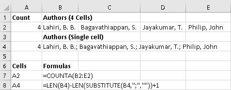
If the Authors are in separate cells use COUNTA, but if the authors are in a single cell use Len(cell) - Len(substitute( method.
(see Figure 1 below)

Figure 1.
2020-01-12 22:39:38
Anirudh Rangarajan
Can you please send me the commands/functions in excel for author count
===============================================
No. of authors in a row is 4
Lahiri, B. B.; Bagavathiappan, S.; Jayakumar, T.; Philip, John = 4
2019-11-17 09:51:17
Paul
J. Wooley, thank you for the last tip. I have used it successfully and will, without a doubt, incorporate it into other projects I am working on.
Peter Atherton, although I wasn't looking for a macro based solution I learned a lot from the one you posted. Thanks.
2019-11-15 11:37:43
J. Woolley
@Paul
Here is another solution to your problem described 2019-11-06. Assuming all of your 200 worksheets have a similar structure, pick an unused column (one that has no values or formulas on any worksheet). Let's assume you picked column Z. Click the first worksheet's tab, then Shift+Click the 200th worksheet's tab; all 200 worksheets should be selected with one of them the active sheet. Put the following 3 formulas in cells Z1, Z2, and Z3 of the active sheet:
=--(UPPER(K16)="R")
=--(UPPER(K16)="L")
=--(UPPER(K16)="C")
Now all 3 formulas should appear in Z1:Z3 on all 200 sheets. Notice these formulas ignore alphabetic case of cell K16, which is optional. The double unary (double negative) operator converts TRUE/FALSE to 1/0.
Now select (activate) your summary sheet and use the following formulas to count the number of sheets that have "r", "l", or "c" in cell K16:
="r count is "&SUM(’Sheet(1):Sheet(200)'!Z1)
="l count is "&SUM(’Sheet(1):Sheet(200)'!Z2)
="c count is "&SUM(’Sheet(1):Sheet(200)'!Z3)
2019-11-14 14:36:02
J. Woolley
@Paul
You might be interested in these articles:
https://ask.wellsr.com/1159/why-is-range-so-different-in-count-and-sum-vs-countif-and-sumif
https://exceljet.net/formula/count-occurrences-in-entire-workbook
2019-11-06 21:36:22
Peter Atherton
Paul
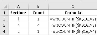
I know that you said no macros but sometimes a VB function leads to Microsoft wizards to write a new function. Here is a UDF to perform the task.
Function wbCOUNTIF(ref, val As String)
Dim addr As String, wks As Worksheet
Dim i As Integer, cnt As Integer
Dim ShCount As Integer, str As Variant
addr = ref.Range("A1").Address
i = 1
ShCount = ThisWorkbook.Sheets.Count
On Error Resume Next
For i = 2 To ShCount
Set wks = Worksheets(i)
With wks
str = wks.Range(addr).Value
If LCase(str) = LCase(val) Then
cnt = cnt + 1
End If
End With
Next i
wbCOUNTIF = cnt
End Function
(see Figure 1 below)

Figure 1.
2019-11-06 14:46:24
J. Woolley
@Paul
Because you originally said "no macros" I assume you don't want a VBA user-defined function (which would be easy to specify). In other words, you want something that can be saved in an XLSX file, not XLSM or XLSB.
First create a list of all your sheet names. For example, put this formula in cell A1
="Sheet("&ROWS($A$1:A1)&")"
then duplicate that formula down the column (range A1:A200).
With the sheet names in A1:A200, these formulas will count the number of sheets that have "r", "l", or "c" in cell K16
=SUMPRODUCT(COUNTIF(INDIRECT("'"&A1:A200&"'!K16"),"r"))
=SUMPRODUCT(COUNTIF(INDIRECT("'"&A1:A200&"'!K16"),"l"))
=SUMPRODUCT(COUNTIF(INDIRECT("'"&A1:A200&"'!K16"),"c"))
2019-11-06 09:02:02
Paul
J. Wooley thank you for your response. This isn’t the problem I’m having. My workbook contains 200 worksheets (each named sheet(1), sheet(2), etc.) containing data and 2 summary pages that collect information from the worksheets. One of the formulas I created in a summary worksheet to total the number of items sold is =SUM(’Sheet(1):Sheet(200)'!F12), where the number is entered in cell F12 on each worksheet. This gives me an instant update when something is sold. I have also used the MAX and MIN functions in a similar fashion for ordering purposes. I keep items stored in 3 sections of a small warehouse that I identify with an r for right side, l for left side, and c for center. This letter (r, l, or c) is located in cell k16 of each worksheet. I want to be able to count the number items I have in each section by simply counting the number r’s, the number of l’s, and the number of c’s using a formula structure similar to what I used above. A formula for each letter would be satisfactory rather than one formula that tries to count each.
2019-11-05 13:10:18
J. Woolley
@Paul
Assuming the specific text character you want to count is in cell A1 (for example, cell A1 contains the text character r) and you want to count the number of times that character appears in cell A5, use the following formula for a count that is alphabetic case sensitive:
=LEN(A5)-LEN(SUBSTITUTE(A5,A1,""))
To ignore alphabetic case, use the following formula:
=LEN(A5)-LEN(SUBSTITUTE(UPPER(A5),UPPER(A1),""))
2019-11-04 14:19:20
Paul
I have a workbook that contains 200 worksheets (sheet(1), sheet(2), etc.) I am trying to find a formula (no macros) that will enable me to count the total number of times a specific text character ( r for example) appears in a specific cell (a5). There are 5 letters that could be in the cell. I have tried variations on "counter", but I can't seem to get the syntax correct.
2016-04-23 05:58:48
Michael (Micky) Avidan
@Amy,
1. Although we don't deal with "life danger" - one should avoid using Absolute references if he deals with a SINGLE formula.
2. the following "shorten" formula will return the same result:
=COUNTIF(A2:B200,"=")
--------------------------
Michael (Micky) Avidan
“Microsoft® Answers" - Wiki author & Forums Moderator
“Microsoft®” MVP – Excel (2009-2016)
ISRAEL
2016-04-22 17:07:18
Amy
Just change the formula such as
=COUNTIF($A$2:$B$200,"="&"")
2016-04-21 16:12:12
Rundor
Is there a way to COUNTIF cells are blank?
2016-04-17 06:25:17
Willy Vanhaelen
@Dave
You're right. This construction is only needed for not equal for instance:
=COUNTIF($A$2:$B$200,"<>"&E2).
2016-04-16 06:45:28
Dave
in the formula
=COUNTIF($A$2:$B$200,"="&$E2)
what is the purpose of "="& as the formula works perfectly well without it?
Got a version of Excel that uses the ribbon interface (Excel 2007 or later)? This site is for you! If you use an earlier version of Excel, visit our ExcelTips site focusing on the menu interface.
FREE SERVICE: Get tips like this every week in ExcelTips, a free productivity newsletter. Enter your address and click "Subscribe."
Copyright © 2026 Sharon Parq Associates, Inc.
Comments