RoseMary has a column of full names in a worksheet. She needs to extract just the initials of the names and add an instance number based on the person to which the initials belong. For example, the list may have Jane Doe twice, but also a Justin Dixon and a John Doe. When the initials are extracted, then all four names would equate to JD. She would need Jane Doe to be JD1, Justin Dixon to be JD2, and John Doe to be JD3, leaving each person with a unique ID.
This is a deceptively tricky problem that RoseMary has. Let's take a look at why this is so. The first thing to do is to derive the initials from the full names in column A. You might think that a formula that pulls the first letter of the cell (A2 in this case), combined with the first letter after the first space, would work, like this:
=LEFT(TRIM(A2),1)&MID(TRIM(A2),FIND(" ",TRIM(A2))+1,1)
This won't necessarily work, however, because RoseMary hasn't defined what is meant by "full names." If it is just first name and surname, then it will work. If, however, a full name includes a middle name, then the function will return the first letters of the first and middle name and not the surname. Things get trickier still if there is a suffix to the name, such as "Sr." or "Jr."
To keep things somewhat simple, we have to make some assumptions about the names. I'll assume that the "full names" can consist of any number of words greater than one, but that the last word won't be a suffix. (In other words, no suffixes in the names.) With this assumption in place, the following formula will construct the two-letter set of initials from the name:
=LEFT(TRIM(A2),1) & LEFT(TEXTAFTER(TRIM(A2)," ",-1),1)
Yes, this formula uses the TEXTAFTER function, which is available (at this point) only in the version of Excel provided with Microsoft 365. Unfortunately, there is no equivalent function or an easily constructed formula that will return the first character after the last space in a text string. In that case it would, in my estimation, be easier to use a macro. (I'll get to that in just a bit.)
If you put this formula into cell B2 and copy it downward, you end up with the two-letter set of initials for each name in column A. At this point you could add another formula in column C that would combine the initials with the instance of each set of initials:
=B2&COUNTIF(B$2:B2,B2)
Copy it downward, and you may think you are done, having your unique ID for each name. This is not true, however. Go back and read what RoseMary said about the names in column A—there can be duplicates. (She specifically mentions a list having "Jane Doe" twice.) And RoseMary wants a unique ID that applies to all occurrences of duplicate names. With the formulas discussed so far, you end up with erroneous IDs. (See Figure 1.)
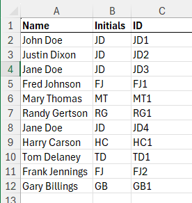
Figure 1. Example data. Notice the different IDs for Jane Doe at cells C4 and C8.
All that we've done so far is to generate an ID that is based on the occurrence of the initials, but it has to take the names in column A into account, as well. The easiest way to do this is to add one more helper column, this one to indicate the instance of the initials. This column (which I'll insert in column C) will use the COUNTIF function to return the instance:
=COUNTIF(B$2:B2,B2)
Now, with this in place and copied downward, the final IDs can be generated in column D with this formula:
=B2&IF(C2>1,XLOOKUP(A2,A$2:A2,C$2:C2),C2)
It checks to see if the instance number (in C2) is greater than 1. If it is, then it uses XLOOKUP to find the first occurrence of the name in column A and then returns the instance number for that occurrence. The correct instance number is what is appended to the initials. (See Figure 2.) Note that this formula uses the XLOOKUP function, which is (again) only available in the latest versions of Excel. I didn't figure it was a big deal at this point since we already limited versions by using the TEXTAFTER function to put the initials together.
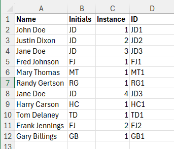
Figure 2. Example data. Notice the proper ID for Jane Doe at cells D4 and D8.
I mentioned earlier that if you were using an earlier version of Excel, it may be easier to simply use a macro to generate the IDs. In fact, you could create a user-defined function that will return the ID you seek. All you need to do is make sure that you pass to the function the range of cells that contain the names and the cell for which you want the ID. Here's an example:
Function UniqueID(ByVal rN As Range, ByVal rNR As Range) As String
    Dim sTemp() As String
    Dim sNames() As String
    Dim iRows As Integer
    Dim r As Range
    Dim J As Integer
    Dim K As Integer
    Dim L As Integer
    Dim bMyError As Boolean

    ' Check that first parameter is a single cell
    ' and that second parameter is only asingle column
    bMyError = False
    If rN.Cells.Count > 1 Then bMyError = True
    If rNR.Columns.Count > 1 Then bMyError = True

    If bMyError Then
        UniqueID = "Problem with parameters"
    Else
        ' Redim array based on number of rows
        iRows = rNR.Rows.Count
        ReDim sTemp(iRows, 2)

        ' Construct array of names and IDs based on instances of initials
        J = 0
        For Each r In rNR.Rows
            J = J + 1
            ' Set first dimension to name
            sTemp(J, 1) = Trim(r.Cells(1))
            ' Set second dimension to initials
            sNames = Split(sTemp(J, 1), " ")
            sTemp(J, 2) = Left(sNames(LBound(sNames)), 1) & Left(sNames(UBound(sNames)), 1)
            ' Append instance number to initials
            K = 0
            For L = 1 To J
                If Left(sTemp(L, 2), 2) = Left(sTemp(J, 2), 2) Then K = K + 1
            Next L
            sTemp(J, 2) = sTemp(J, 2) & K
        Next r

        ' Based on name, return first ID
        UniqueID = ""
        For J = 1 To iRows
            If Trim(rN.Cells(1)) = sTemp(J, 1) Then
                UniqueID = sTemp(J, 2)
                Exit For
            End If
        Next J
    End If
End Function
I have no doubt that the macro could be shortened, but it does the trick. Plus, as written, it is relatively easy to understand what it is doing. You use it in your worksheet using this formula:
=UniqueID(A2,A$2:A$12)
The first parameter is the single cell for which you want the ID and the second parameter is the range of cells that contain all of the names. The function ignores multiple spaces in names and, as discussed, constructs the two-letter initials using the first and last names in a cell.
ExcelTips is your source for cost-effective Microsoft Excel training. This tip (13928) applies to Microsoft Excel 2007, 2010, 2013, 2016, 2019, 2021, and Excel in Microsoft 365.

Best-Selling VBA Tutorial for Beginners Take your Excel knowledge to the next level. With a little background in VBA programming, you can go well beyond basic spreadsheets and functions. Use macros to reduce errors, save time, and integrate with other Microsoft applications. Fully updated for the latest version of Office 365. Check out Microsoft 365 Excel VBA Programming For Dummies today!
If you have a lot of values in a single row, you might want to pull the last non-zero value from that row. There are a ...
Discover MoreWant to add up a bunch of scores, without including the lowest one in the bunch? You can make a small change to your ...
Discover MoreWhen processing some text data, you may need to perform some esoteric function, such as adding dashes between letters. ...
Discover MoreFREE SERVICE: Get tips like this every week in ExcelTips, a free productivity newsletter. Enter your address and click "Subscribe."
2024-07-08 19:33:22
Debbie
This looks like it will be helpful to me. My guidelines are slightly different. I want Last Name and First Initial and 1 or whatever is the ordinal number for this name. A difference is that it is a constantly growing list. If 2 is already taken, the new one needs to be 3, even if it is alphabetically earlier. I'm thinking I will need to go with the formula option.
2024-07-08 11:36:09
J. Woolley
@Erik
You make a good point, but I'll assume RoseMary wants the IDs to be recalculated after any change to the column of names. Notice she did not specify a limit on the number of characters for initials. The solution in my previous comment below assumed two characters, but since names might have more than two words I now believe the initials should take the first character of each word.
To list initials with an instance number for the names in column A without incrementing the instance number for a given name, put this formula in cell B2 and copy down column B:
=LET(name, TRIM(A19), id, VLOOKUP(name, TRIM($A$1:B18), 2, FALSE),
chars, LEFT(TEXTSPLIT(name," "), 1), initials, CONCAT(chars),
uniq, UNIQUE(B$1:B18), digits, RIGHT(uniq, 2),
previous, LEFT(uniq, LEN(uniq)-IF(ISERROR(INT(digits)), 1, 2)),
IF(ISNA(id), initials&SUMPRODUCT(--(previous=initials))+1, id))
This formula does not require a helper column, but it does require the LET and UNIQUE functions in Excel 2021. It also uses TEXTSPLIT which currently requires Excel 365, but the SplitText function in My Excel Toolbox can be substituted; see my comment here: https://excelribbon.tips.net/T009396
This formula accommodates up to 99 different names that have the same initials (instance numbers 1 to 99). (see Figure 1 below)
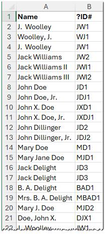
Figure 1.
2024-07-06 17:17:15
Erik
The problem with the formula method is that, since the IDs are live, many actions will change some users' IDs. Examples include sorting the list in alphabetical order; deleting someone from the list; adding or removing rows from the middle of the list; revising a name, for example due to marriage/divorce (unless a new ID is intended with any name change); etc.
While I am not familiar with macros or Power Query, I suspect they could be written to avoid this problem.
2024-07-06 11:46:50
J. Woolley
The Tip has its simplifying assumptions; here are mine (no middle names):
1. Cell A1 is a one-word header (such as “Names”)
2. Column A lists full names starting in row 2
3. Each full name in column A consists of two words (first and last names)
4. First and last names begin with alphabetic characters (A-Z or a-z)
5. Column A might have extraneous space characters before/after/between first and last names
6. Cell B1 is a header that must NOT begin with an alphabetic character (such as “??#”)
To list initials with an instance number for the names in column A (such as “JD1”) without incrementing the instance number for a given name, put this formula in cell B2 and copy down column B:
=LET(name, TRIM(A2), id, VLOOKUP(name, TRIM($A$1:B1), 2, FALSE),
initials, LEFT(name, 1)&MID(name, FIND(" ", name)+1, 1),
IF(ISNA(id), initials&(COUNTIF(B$1:B1, initials&"*")+1), id))
This formula requires the LET function in Excel 2021 or later. It does not require a helper column.
2024-07-06 08:58:39
Ron S
I would suggest using similar logic in Power query instead.
.
Once you figure out the logic, PQ builds most of the ("macro") code for you in the background. It lets you see the results, and mistakes in logic, immediately. Much easier to debug than macros because the results are shown immediately.
Macros are OK for simple logic, but PQ is better suited for complex logic. You can use the user interface to build simple code, the manually edit it, like macro code, to make it more complex and more generic. There are lots of sites that provide PQ training and tips.
Macros are the past. PowerQuery is a skill you need be relevant in the future! To maximize your earning potential in the future.
Got a version of Excel that uses the ribbon interface (Excel 2007 or later)? This site is for you! If you use an earlier version of Excel, visit our ExcelTips site focusing on the menu interface.
FREE SERVICE: Get tips like this every week in ExcelTips, a free productivity newsletter. Enter your address and click "Subscribe."
Copyright © 2026 Sharon Parq Associates, Inc.
Comments