Locating a Single-Occurrence Value in a Column

Bill has a column of numbers sorted in ascending order. There are many duplicate values within the column, which is just fine. However, he needs to locate the first instance of a number in the column that does not have a duplicate. Bill wonders if there is a formula that could identify the first single-occurrence value in the column.

There are quite a few ways that the desried answer could be found. One way is to add a helper column to the right of your numbers. Assuming that your first number is in cell A2, you could enter the following in cell B2:

=IF(AND(A1<>A2,A3<>A2),"single","")

Copy the formula down as many cells as necessary and you'll be able to easily spot the first cell that has a single value in column A.

You could also use the following formula in cell B2:

=COUNTIF($A:$A,$A2)

Copy it down as far as necessary; the formula shows a count of the number of times the value in column A occurs within column A. You would then use the following formula to determine the first value that occurs once in column A:

=INDEX($A:$A,MATCH(1,$B:$B,0))

If a helper column is not possible, you could rely on array formulas. Either of these will show the first value that occurs a single time:

=INDEX(A2:A999,MATCH(1,COUNTIF(A2:A999,A2:A999),0))
=SMALL(IF(COUNTIF(A2:A999,A2:A999)=1,A2:A999,""),1)

Remember that these are array formulas, which means you need to enter them by using Ctrl+Shift+Enter. Plus, if there is no single value within the range, the formula returns an #N/A error.

If you wanted to know which row contained the first single-occurrence value, the following array formula will do nicely:

=MATCH(1,COUNTIF(A2:A999,A2:A999),0)+1

Note that the formula checks cells A2:A999. Since row A1 is skipped, the "+1" is required at the end of the formula. If you have no header row, or if your data starts in a row other than row 2, you'll want to adjust the formula accordingly.

If you don't want to use a formula, you can highlight the single-occurrence values in your data by using Conditional Formatting. Follow these steps:

1. Select the cells you want to check.
2. With the Home tab of the ribbon displayed, click the Conditional Formatting option in the Styles group. Excel displays a palette of options related to conditional formatting.
3. Choose Highlight Cells Rules. Excel displays even more options.
4. Choose Duplicate Values. Excel displays the Duplicate Values dialog box. (See Figure 1.)



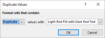
Figure 1. The Duplicate Cells dialog box.

5. Using the drop-down list at the left of the dialog box, choose Unique.
6. Use the drop-down list at the left of the dialog box to indicate how you want the single-occurrence values formatted.
7. Click OK.

At this point your single-occurrence values are formatted as you specified in step 6, and you can easily spot them. If you want to see only the single-occurrence values, after applying the Conditional Format you can use filtering to accomplish the task.

If you prefer a macro approach, then you could use a macro such as the following:

Sub FirstUnique()
    Dim c As Range
    Dim sMsg As String
    Dim bLone As Boolean

    If Selection.Cells.Count > 1 Then
        For Each c In Selection.Cells
            bLone = False
            If c.Row = 1 Then
                If c <> c.Offset(1, 0) Then bLone = True
            Else
                If c <> c.Offset(-1, 0) And _
                   c <> c.Offset(1, 0) Then bLone = True
            End If
            If bLone Then
                sMsg = "First single-occurrence value found "
                sMsg = sMsg & "at " & c.Address & vbCrLf
                sMsg = sMsg & "Value: " & c
                MsgBox sMsg
                Exit For
            End If
        Next c
    Else
        sMsg = "You must select at least 2 cells."
        MsgBox sMsg
    End If
End Sub

In order to use the macro, select the cells you want to check and then run it. The macro displays the address and value of the first single-occurrence value in your selection.

ExcelTips is your source for cost-effective Microsoft Excel training. This tip (3383) applies to Microsoft Excel 2007, 2010, 2013, 2016, 2019, 2021, and Excel in Microsoft 365.