Determining a Name for a Week Number

Theo uses an Excel worksheet to keep track of reservations in his company. The data consists of only three columns. The first is a person's name, the second the first week number (1-52) of the reservation, and the third the last week number of the reservation. People can be reserved for multiple weeks (i.e., start week is 15 and end week is 19). Theo needs a way to enter a week number and then have a formula determine what name (column A) is associated with that week number. The data is not sorted in any particular order, and the company won't let Theo use a macro to get the result (it has to be a formula).

Theo's situation sounds simple enough, but it is filled with pitfalls when devising a solution. Looking at the potential data (as shown in the following figure) quickly illustrates why this is the case. (See Figure 1.)

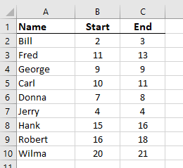
Figure 1. Potential data for Theo's problem.

Notice that the data (as Theo said) is not in any particular order. Note, as well, that there are some weeks where there are no reservations (such as week 5 or 6), weeks where there are multiple people (such as week 11 or 16), and weeks where there is someone reserved, but the week number doesn't show up in column B or C (such as week 12 or 17).

Before starting to look at potential solutions, let's assume that the week you want to know about is cell E1. You should name this range as Query. Further, name the range that contains people's names (in this example, cells A2:A10) as ResNames, the starting weeks (B2:B10) as StartWeeks, and the ending weeks (C2:C10) as EndWeeks. Finally, define a name for the entire table (A2:C10), such as MyData. This naming, while not strictly necessary, will make understanding the formulas much easier.

One potential solution is to add what is commonly referred to as a "helper column." Add the following to cell D2:

=IF(AND(Query>=B2,Query<=C2),"RESERVED","")

Copy the formula down, for as many cells as there are names in the table. (For example, copy it down through cell D10.) When you place a week number in cell E1, then the word "RESERVED" appears to the right of any reservation that involves that week number. It is also easy to see if there are multiple people reserved for that week or if there are no people reserved for that week. You could even apply an AutoFilter and select to only show those records with the word "RESERVED" in column D.

You can, if desired, forego the helper column and consider using conditional formatting to display who is reserved for a desired week. Simply select the names in column A and add a conditional formatting rule that uses the following formula:

=AND(Query>=B2,Query<=C2)

(How you enter conditional formatting rules has been described extensively in other issues of ExcelTips.) Set the rule so that it changes the shading (pattern) applied to the cell, and you'll easily be able to see which reservations apply to the week you are interested in.

Another approach is to use an array formula. Select a few more cells than the number of overlapping reservations you expect, and then enter the following into those cells by pressing Ctrl+Shift+Enter:

=IFERROR(INDEX(ResNames,LARGE((StartWeeks<=Query)*(EndWeeks>=Query)*(ROW(ResNames)),ROW()-1)-1),"")

When picking the number of cells, you want this array formula to occupy, look at, for instance, the number of people that may be reserved over week 11. In the example shown in this tip, it is 2 people. Select more than that number of cells and then put the array formula in those cells. If you expect that you might have 20 people potentially booked for the same week, then you'll want to pick a larger number of cells, such as 20 or 30. Just select the cells, put the formula in the Formula bar, and then press Ctrl+Shift+Enter.

Finally, you really should consider revising how your data is laid out. You could create a worksheet that has week numbers in column A (1 through 52 or 53) and then place names in column B. If a person was reserved for two weeks, their name would appear in column B twice, once beside each of the two weeks that they reserved.

With your data in this format, you could easily scan the data to see which weeks are available, which are taken, and who they are taken by. If you want to do some sort of lookup, it is easy to use the VLOOKUP function based on the week number, since it is the first column of the data, in sorted order.

ExcelTips is your source for cost-effective Microsoft Excel training. This tip (11078) applies to Microsoft Excel 2007, 2010, 2013, 2016, 2019, and Excel in Microsoft 365. You can find a version of this tip for the older menu interface of Excel here: Determining a Name for a Week Number.