Written by Allen Wyatt (last updated April 18, 2020)
This tip applies to Excel 2007, 2010, 2013, 2016, 2019, and 2021
Om has hundreds of differently named worksheets all in the same workbook. The structure of each worksheet is essentially the same. He wants to copy a fixed range (A146:O146) from each worksheet to a new worksheet, one row after another.
There are a few ways you can go about doing this. For my money, a simple macro is the best bet. Before getting into the macro-based approach, however, there is a way you can do it using formulas. One rather unique way relies upon defining a formula in the Name Manager. Follow these steps to start:
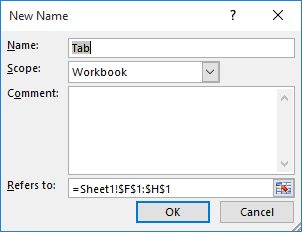
Figure 1. The New Name dialog box.
=REPLACE(GET.WORKBOOK(1),1,FIND("]",GET.WORKBOOK(1),1),"")
With the formula defined in this way, you can then go to the worksheet on which you want to amalgamate all those ranges. (Let's say that the name of this worksheet is "Summary.") I strongly suggest making sure this worksheet is the very last one in your workbook. On the Summary worksheet, put the following formula in column A of any row:
=INDIRECT(INDEX(ListSheets,ROWS($A$1:$A1))&"!"&CELL("address",A$146))
Copy the formula down however many rows are necessary to represent all the worksheets. In other words, if you have 25 worksheets (not counting the Summary worksheet), copy the formula down 24 rows. Counting the original, you should now have the formula appear in a total of 25 rows.
A side note here: The ListSheets formula—the one you defined in the Name Manager—returns an array of worksheet names. The ROWS function is used to determine which element of that array is returned through the INDEX function. If your Summary worksheet is not the last one in your workbook, it can easily be returned by ListSheets and you will end up pulling values from it. This is undoubtedly something you don't want to do, which is why I suggested making sure Summary was the last worksheet in the workbook.
Now simply copy the formulas from column A to the right so that you have them all the way through column O. The result is that you will have the values from A146:O146 in the cells containing the formulas.
Earlier I said that I think a macro-based approach is the best bet. Here's a short little macro that demonstrates why this is the case.
Sub CopyRange()
    Dim w As Worksheet
    Dim sRange As String
    Dim lRow As Long

    sNewName = "Summary" 'Name for summary worksheet
    sRange = "A146:O146" 'Range to copy from each worksheet

    Worksheets(1).Select
    Worksheets.Add
    ActiveSheet.Name = sNewName

    lRow = 2
    For Each w In Worksheets
        If w.Name <> sNewName Then
            'Comment out the following line if you don't want to
            'include worksheet names in the summary sheet
            Cells(lRow, 1) = w.Name
            'If you commented out the previous line, make a change
            'in the following line: change (lRow, 2) to (lRow, 1)
            w.Range(sRange).Copy Cells(lRow, 2)
            lRow = lRow + 1
        End If
    Next w
End Sub
Note that there are two variables (sNewName and sRange) that are set at the beginning of the macro. These represent the name you want used for the new summary worksheet created by the macro and the range of cells you want to copy from each worksheet.
The macro then makes the first worksheet in the workbook active and adds a new worksheet to be used for summarization. This worksheet is assigned whatever name you specified in the sNewName variable. The macro then steps through a loop checking each of the other worksheets. As long as the worksheet isn't the summary one, then the name of the worksheet is placed into column A of the summary sheet and the range specified in the sRange variable (A146:O146) is copied to the summary worksheet starting at column B.
The macro approach is fast and easy. Plus, if you ever need to redo your summary sheet, just delete the old one and rerun the macro.
Note:
ExcelTips is your source for cost-effective Microsoft Excel training. This tip (9812) applies to Microsoft Excel 2007, 2010, 2013, 2016, 2019, and 2021.

Best-Selling VBA Tutorial for Beginners Take your Excel knowledge to the next level. With a little background in VBA programming, you can go well beyond basic spreadsheets and functions. Use macros to reduce errors, save time, and integrate with other Microsoft applications. Fully updated for the latest version of Office 365. Check out Microsoft 365 Excel VBA Programming For Dummies today!
Macros often need to select different cells in a worksheet. Here's how you can use macro commands to change which cell is ...
Discover MoreWhen you assign a macro to a shortcut key, you make it easy to run the macro without ever removing your hands from the ...
Discover MoreDoes your macro need to get some input from a user? Here are the ways that Excel provides for that input to be solicited.
Discover MoreFREE SERVICE: Get tips like this every week in ExcelTips, a free productivity newsletter. Enter your address and click "Subscribe."
2022-05-06 08:30:48
Alex Blakenburg
@Katie, You're welcome. Glad I could help.
2022-05-06 05:24:35
Katie
Perfect! Thanks so much Alex :)
2022-05-05 04:50:34
Alex Blakenburg
@Katie, I think there is an issue with the code and the copies are overlapping each other leaving only the first row visible except for the last copy which has no others being copied over the top.
Change this line
lRow = lRow + 1
to this
lRow = lRow + w.Range(sRange).rows.count
so that you are advancing the row counter by the no of lines being copied in.
2022-05-05 00:44:17
Katie
Hi Allen,
Thanks so much for posting this macro, it works almost perfectly for what I need to do however I am having a slight issue with it...
My range of cells copying from each sheet is L2:N4. So that's 3 columns across and 3 rows down. I have over 1000 worksheets in my actual data so am just testing it with 5 for the moment. When I run the Macro, the Summary for some reason is only copying the first row for the first 4 worksheets however on the 5th worksheet it copies over all 3 rows.
The data is in the same format for all 5 worksheets so I cant figure out why this is happening. Any advice would be very much appreciated.
Thanks
Katie :)
2020-04-19 10:37:10
Alex B
Oops item 1 in my previous comment should read:
Dim sNewName
2020-04-18 22:42:34
Alex B
The macro above has a couple of errors in it:
1) Add the following statement
sNewName
(most people will have Option Explicit set and this name needs to be defined)
2) Assuming A146:O146 has formulas in it, your copy results will come back with #REF!
since the formulas won't work in the new location
• Replace
w.Range(sRange).Copy Cells(lRow, 2)
• With
w.Range(sRange).Copy
' Paste the data
Cells(lRow, 2).PasteSpecial xlPasteValues
' Turn off copy selection
Application.CutCopyMode = False
2020-04-18 05:14:58
Rene
There is also another method. On your summary sheet you can have the first column contain the names of the tabs. In each row, use the "Indirect" function to copy from each tab. The easiest way to do this is to fill the first cell with the reference you want to copy from e.g. from the above example, in cell B1, you would have the formula ={tab} A$146. Now change the formula to Indirect and have {tab} refer to the tab name in A1 ($A1). This will give you the result of Tab cell A146. The formula can be copied down and to the right. New rows can be added, all you need to do is change the tab name.
If you want to show various cells which aren't next to each other, you can add a line at the top where you show the column which needs to be selected. The formula should then also refer to the column on row 1 to pick up the column reference.
This can be expanded as much as you want, adding reference lines or columns to allow selection of any cell in a tab. This method of indirect function makes it clearer for the user where information comes from.
Got a version of Excel that uses the ribbon interface (Excel 2007 or later)? This site is for you! If you use an earlier version of Excel, visit our ExcelTips site focusing on the menu interface.
FREE SERVICE: Get tips like this every week in ExcelTips, a free productivity newsletter. Enter your address and click "Subscribe."
Copyright © 2026 Sharon Parq Associates, Inc.
Comments