Preventing Automatic Date Formatting Changes

In a worksheet, Carol has a cell formatted to "Accounting." If someone accidentally enters a date (mm/dd/yy) in that cell, Excel automatically changes the formatting of the cell to show the date correctly. However, if she tries to enter a dollar amount in that cell again, it will not go back to the "Accounting" format; the cell remains in the date format. This is fine if the user sees the error and corrects it, but many times this is happening in a template with "boilerplate" text and the template is protected with no access to formatting cells. Carol wonders if anyone has any ideas on why this happens and how to correct it.

If you want a quick way to prevent the formatting change in simple worksheets, follow these steps:

1. Display the Excel Options dialog box. (In Excel 2007 click the Office button and then click Excel Options. In Excel 2010 or a later version display the File tab of the ribbon and then click Options.)
2. At the left side of the dialog box click Advanced.
3. Scroll to the very bottom of the advanced options. (See Figure 1.)



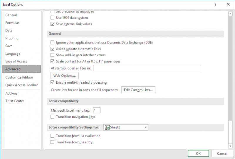
Figure 1. The Advanced options in the Excel Options dialog box.

4. Make sure the Transition Formula Entry option is selected.
5. Click OK.

This particular option causes Excel to evaluate (parse) entered information in the same way that Lotus 1-2-3 did. This means that dates are no longer parsed as dates, but as a formula. Thus, if someone enters 11-16-13 into a cell, then it is parsed as "eleven minus sixteen minus thirteen" and shown in the cell as -18. Because it was not parsed as a date, then the Accounting format is left associated with the cell, as desired.

There are drawbacks to this approach, though. Because Excel subsequently parses any entries according to Lotus rules, your users may conclude that your worksheet doesn't work properly since it doesn't follow the same rules that other Excel worksheets do. This is why I mentioned that this approach may be acceptable for simple worksheets; you'll need to make the determination if your worksheet qualifies.

If you don't want to change how parsing is done, the best approach may be to add some event handlers to your worksheet. For instance, you could include an event handler that looks at where data was entered and ensures that any changes to those cells retain the desired formatting.

Private Sub Worksheet_Change(ByVal Target As Range)
    Dim rngToCheck As Range
    Set rngToCheck = Range("E2")
    If Intersect(Target, rngToCheck) Then
        rngToCheck.NumberFormat = _
          "_($* #,##0.00_);_($* (#,##0.00);_($* "" - ""??_);_(@_)"
    End If
End Sub

In this example, the cell that you want to retain the Accounting format in is E2, as assigned to the rngToCheck variable. If you want to force the format on a different cell range, then just change the assignment line.

If you wanted a bit more flexibility, then you could use a different set of event handlers. For instance, the following examples use both the SelectionChange and Change events of the Worksheet object. They result in something that doesn't so much force a particular format, but it prevents the formatting of a cell from being changed from whatever it was before. Thus, this approach protects any formatting, not just enforcing an Accounting format.

Dim nFormat As String

Private Sub Worksheet_Change(ByVal Target As Range)
    Dim rngToCheck As Range
    Set rngToCheck = Range("E2")
    If Intersect(Target, rngToCheck) Then
        rngToCheck.NumberFormat = nFormat
    End If
End Sub

Private Sub Worksheet_SelectionChange(ByVal Target As Range)
    nFormat = Target.NumberFormat
End Sub

The SelectionChange event handler fires first, setting the existing format into the nFormat variable. Then the Change event handler fires and sets the formatting back to the original.

Another approach you could try is to use data validation. This approach doesn't require any macros and is therefore suitable if your workbook will be used by people who may have macros disabled on their system. Follow these general steps:

1. Select the cell or cells whose formatting you want to enforce.
2. Display the Data tab of the ribbon.
3. Click the Data Validation tool in the Data Tools group. Excel displays the Data Validation dialog box.
4. Using the Allow drop-down list, choose Custom. (See Figure 2.)



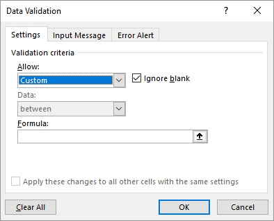
Figure 2. The Data Validation dialog box.

5. In the Formula box, type the following: =CELL("format",B2)="C2"
6. Set any other data validation settings as desired.
7. Click OK.

The formula (step 5) checks the formatting of the cell and either allows or disallows entry based on that formatting. In the formula as cited, format C2 is the internal name for the Accounting format. You could easily change the codes in the formula to some other format, such as ",2", "C2", "C0", "C2-", or "C0-" depending on your preference. The easiest way to figure out what format you should use is to format a cell, as desired, before applying the data validation rule. (For instance, let's say you apply the formatting to cell L13.) You can then use this formula in a different cell to see what format Excel believes you've applied:

=CELL("format",L13)

ExcelTips is your source for cost-effective Microsoft Excel training. This tip (12729) applies to Microsoft Excel 2007, 2010, 2013, 2016, 2019, and Excel in Microsoft 365.