Written by Allen Wyatt (last updated April 29, 2023)
This tip applies to Excel 2007, 2010, 2013, 2016, 2019, 2021, and Excel in Microsoft 365
Excel includes a powerful feature that allows you to format the contents of a cell based on a set of conditions that you specify. This is known as conditional formatting. How you define conditional formats depends on whether you want to define a single formatting condition or multiple conditions. Even if you decide you want to define multiple conditions, however, it is beneficial to understand how single conditions are defined.
The first step in using conditional formatting, of course, is to select the cell whose formatting should be conditional. Then, with the Home tab of the ribbon displayed, click Conditional Formatting in the Styles group. Excel displays a list of various conditions you can define:
In reality, each "condition" selected from these options is nothing but a shortcut to filling in the settings of the New Formatting Rule dialog box. You may have noticed that each of the above choices leads to a series of specific conditions, and that the last condition, in all cases, is "More Rules." If you select this option, if you select one of the defined conditions, or if you select New Rule (available when you first click Conditional Formatting) you will typically see the New Formatting Rule dialog box. (See Figure 1.)
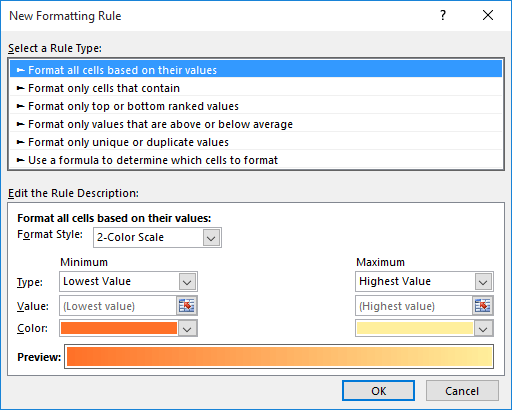
Figure 1. The New Formatting Rule dialog box.
In the top of the dialog box you select a type of rule you want applied to the selected cells. There are six rule types:
These six rule types may look somewhat familiar; they are the basis for the pre-defined rules discussed earlier in this tip. When you select a rule type, Excel changes the settings you can make in the bottom of the dialog box. Each rule type has value, but you will find, over time, that the last rule type (where you use a formula to define formatting) is the most powerful.
When you select a rule type and then adjust the settings in the bottom of the dialog box, you can (depending on the rule type) click the Format button to specify the formatting Excel should apply if the conditions detailed in the rule are satisfied.
When you are satisfied with your rule settings and formatting options, you can click OK to dismiss the New Formatting Rule dialog box. The format is applied and you can continue working in your worksheet.
ExcelTips is your source for cost-effective Microsoft Excel training. This tip (6754) applies to Microsoft Excel 2007, 2010, 2013, 2016, 2019, 2021, and Excel in Microsoft 365.

Best-Selling VBA Tutorial for Beginners Take your Excel knowledge to the next level. With a little background in VBA programming, you can go well beyond basic spreadsheets and functions. Use macros to reduce errors, save time, and integrate with other Microsoft applications. Fully updated for the latest version of Office 365. Check out Microsoft 365 Excel VBA Programming For Dummies today!
Conditional formatting does not allow you to change the typeface and font size used in a cell. You can write your own ...
Discover MoreIf you need to shade alternating rows in a data table, you'll want to examine how you can accomplish the task with ...
Discover MoreIf you have a data table in a worksheet, and you want to shade various rows based on whatever is in the first column, ...
Discover MoreFREE SERVICE: Get tips like this every week in ExcelTips, a free productivity newsletter. Enter your address and click "Subscribe."
There are currently no comments for this tip. (Be the first to leave your comment—just use the simple form above!)
Got a version of Excel that uses the ribbon interface (Excel 2007 or later)? This site is for you! If you use an earlier version of Excel, visit our ExcelTips site focusing on the menu interface.
FREE SERVICE: Get tips like this every week in ExcelTips, a free productivity newsletter. Enter your address and click "Subscribe."
Copyright © 2026 Sharon Parq Associates, Inc.
Comments