Hiding Individual Cells

Ruby has a worksheet that she needs to print out in a couple of different ways, for different users. Part of preparing her data for printing involves hiding or displaying some rows and some columns, as appropriate. Ruby wondered if there was a way to hide the contents of individual cells, as well.

If, by "hide," you want to have the cell disappear and information under it move up (like when you hide a row) or move left (like when you hide a column), then there is no way to do this in Excel. Actual hiding in this manner can only be done on a row or column basis.

There are ways that you can hide the information in the cell, however, so that it doesn't show up on the printout. One easy way, for instance, is to format the cell so its contents are white. This means that, when you print, you'll end up with "white on white," which is invisible. Test this solution, though—some printers, depending on their capabilities, will still print the contents.

If this approach works for you, you could expand on it just a bit to make your data preparation tasks just a bit easier. Follow these general steps:

1. In an out-of-the-way cell (let's say it is cell J1) insert the letter "p."
2. Select the cell (or cells) you want to hide on the printout.
3. With the Home tab of the ribbon displayed, click the Conditional Formatting option in the Styles group. Excel displays a palette of options related to conditional formatting.
4. Click New Rule. Excel displays the New Formatting Rule dialog box.
5. In the Select a Rule Type area at the top of the dialog box, choose Use a Formula to Determine Which Cells to Format. (See Figure 1.)



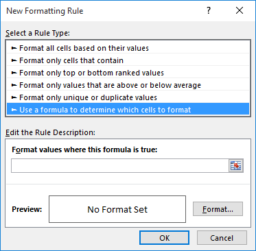
Figure 1. The New Formatting Rule dialog box.

6. In the criteria area for the rule enter the following: =$J$1="p". This formula will return True if the cell contains a lowercase letter "p."
7. Click the Format button. Excel displays the Format Cells dialog box.
8. Make sure the Font tab is displayed. (See Figure 2.)



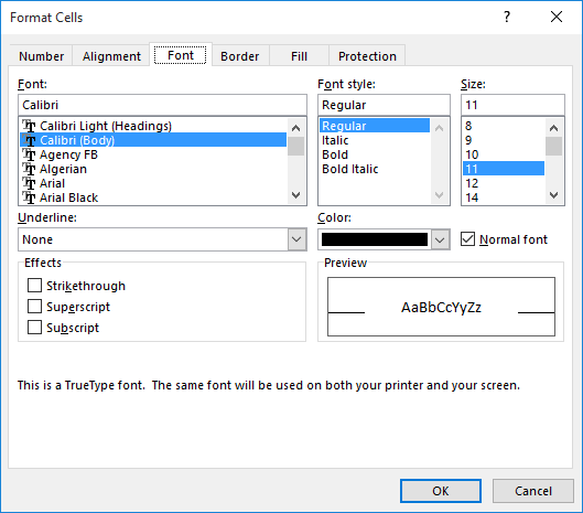
Figure 2. The Font tab of the Format Cells dialog box.

9. Use the Color drop-down list to choose white.
10. Click OK to dismiss the Format Cells dialog box.
11. Click OK to dismiss the New Formatting Rule dialog box.
12. Print your worksheet as normal. The cell contents should not show up on the printout.
13. To make the cell contents visible on the printout, just modify cell J1 so that it contains something other than the letter "p."

Another solution is to use a custom format for the cells whose content you want to hide. Follow these steps:

1. Select the cell (or cells) you want to hide.
2. Display the Home tab of the ribbon.
3. Click the small icon at the lower-right corner of the Number group. Excel displays the Format Cells dialog box.
4. Make sure the Number tab is displayed.
5. In the list of format categories, select Custom. (See Figure 3.)



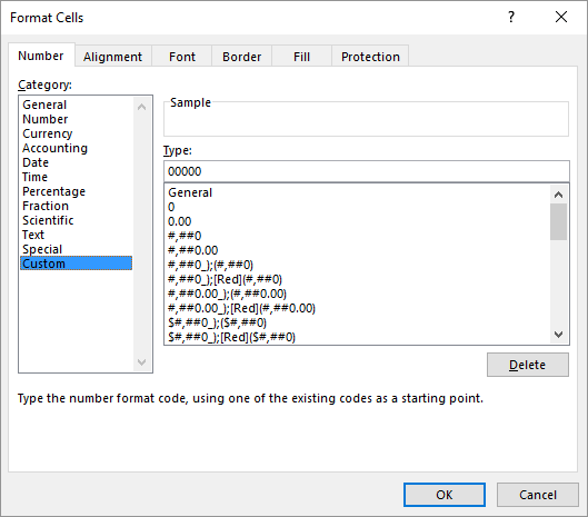
Figure 3. The Number tab of the Format Cells dialog box.

6. In the Type box, enter three semicolons (;;;).
7. Click on OK.

Now the information in the cell is not visible, nor will it print. You can, however, see the information in the Formula Bar, and it can be overwritten if you enter anything else in the cell.

ExcelTips is your source for cost-effective Microsoft Excel training. This tip (6866) applies to Microsoft Excel 2007, 2010, 2013, 2016, 2019, 2021, and Excel in Microsoft 365. You can find a version of this tip for the older menu interface of Excel here: Hiding Individual Cells.