Written by Allen Wyatt (last updated November 2, 2024)
This tip applies to Excel 2007, 2010, 2013, 2016, 2019, 2021, and Excel in Microsoft 365
In cell A1 Marius has the text value "0E11" and in cell A2 he has the text value "0E99". (Both have an apostrophe in front of them and the cells are formatted as Text.) In cell B1 he has 2 and in cell B2 has 4. If Marius uses the formula =SUMIF(A1:A2,"0E99",B1:B2), Excel always returns 6 when it should return 4. It seems that SUMIF is evaluating the parameters as numeric values instead of as the text they are, so Marius wonders how to force Excel to treat them as text.
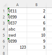
First, let's look at the data, but I'll add a couple more rows. (See Figure 1.)

Figure 1. Data for use with the SUMIF function.
Consider the following formula, referencing this data:
=SUMIF(A1:A7,123,B1:B7)
If any cells in A1:A7 contain the numeric value 123, then the corresponding cells in the range B1:B7 are summed. In this case, only a single cell in A1:A7 (cell A7) contains the value 123, so the value of the corresponding cell in B1:B7 (cell B7) is returned, a sum of 3.
The SUMIF function will work just fine with text values, as well. So, consider this formula referencing the same data:
=SUMIF(A1:A7,"abc",B1:B7)
Again, a single cell (A4) contains "abc", so the value of the corresponding cell (B4) is summed, returning 8.
It is a different story, as Marius discovered, if the text value starts with the characters "0E". The following formula returns a sum of 0, even though it should return a sum of 13:
=SUMIF(A1:A7,"0E99",B1:B7)
It is important to emphasize that this only happens if the leading characters are "0E" followed by one or two digits. Thus, the wrong summing occurs if the match is "0E9" or "0E99", but not if you are matching "0E999" or "1E12". Both of these are treated as text and not converted to numeric values.
The reason for this is that the SUMIF function (and, incidentally, the SUMIFS function) automatically convert text values to numeric values, if it is possible to do so. It apparently does this for both the comparison range (A1:A7) and for the comparison value. You can see this if I revisit a formula used just a moment ago, but with one small change:
=SUMIF(A1:A7,"123",B1:B7)
Notice that I put the comparison value in quote marks ("123"), which one could reasonably think would make Excel treat it as a text value. It does not, however, as the summation produces the same result as if the quote marks were not used.
That, of course, brings us back to the problem expressed by Marius—how to make sure that SUMIF utilizes text values as one would expect. One way, of course, is to simply make some change to the values in A1:A7 so that they couldn't be construed as numeric values. For instance, for each of the cells that begins with "E0" you could pre-pend another character, such as "x" or "n" or just about anything. This is then easier for SUMIF to match without the potential for confusion.
Another approach is to make it clear to SUMIF that you are dealing with text. The easiest way to do this is to include, in the comparison value, a wildcard character. For instance, you could use this:
=SUMIF(A1:A7,"?E99",B1:B7)
This matches anything in A1:A7 that has anything in the first character position and ends in "E99". This will work just fine for "0E99", but it would also match "1E99" or "vE99" or "_E99". If this causes an issue, then this use of a wildcard will work, as well:
=SUMIF(A1:A7,"*0E99",B1:B7)
The asterisk matches multiple characters, or no characters at all. So, it matches "0E99" just fine and returns the proper sum. If you had entries that included a bunch of characters followed by "0E99", then this approach would not be appropriate for your needs, and you'll need to go back to using the question-mark approach.
Of course, Excel provides multiple ways to get the results you want, so depending on your data (as in Marius' case), you may want to use a different function. This will provide the correct summation:
=SUM(B1:B7*(A1:A7="0E99"))
That is because the SUM function doesn't do any conversion of text to numeric values. If using older versions of Excel, you'll need to enter this as an array formula (Ctrl+Shift+Enter). If you want a non-array approach, you can use the SUMPRODUCT function in your formula:
=SUMPRODUCT(B1:B7*(A1:A7="0E99"))
ExcelTips is your source for cost-effective Microsoft Excel training. This tip (7009) applies to Microsoft Excel 2007, 2010, 2013, 2016, 2019, 2021, and Excel in Microsoft 365.

Dive Deep into Macros! Make Excel do things you thought were impossible, discover techniques you won't find anywhere else, and create powerful automated reports. Bill Jelen and Tracy Syrstad help you instantly visualize information to make it actionable. You�ll find step-by-step instructions, real-world case studies, and 50 workbooks packed with examples and solutions. Check out Microsoft Excel 2019 VBA and Macros today!
Need to know what day of the year a certain date is? You can figure it out easily using the formulas in this tip.
Discover MoreWhen you use a function like SUM, you expect it to do its job and return the total for a range of cells. If it doesn't ...
Discover MoreIf you need to change the case of letters in a cell, one of the functions you can use is the PROPER function. This tip ...
Discover MoreFREE SERVICE: Get tips like this every week in ExcelTips, a free productivity newsletter. Enter your address and click "Subscribe."
2024-11-05 09:20:25
J. Woolley
My most recent comment below was directed at Ruth Engle in response to her comment/question. I don't know what happened to @Ruth Engle, which I intended to start with.
2024-11-04 13:00:59
J. Woolley
Apparently the Filter and Advanced Filter features of the Data Ribbon only apply down columns, but you can do this to filter across columns:
1. Select the range to filter; do not include a column containing row headers. (You might want to copy the selected range somewhere in case you need to restore it later.)
2. Pick Data > Sort & Filter > Sort (Alt+A+SS), then Options (O) and Sort Left to Right (L), then Sort By parameters.
3. After sorting the range, hide columns you want to filter out.
To restore the original, use Undo (Ctrl+Z). (If this is not practical, see item 1.)
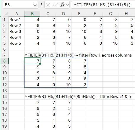
You can also use the FILTER function in Excel 2021 or later to return a filtered range which spills from the formula's cell (not in-place). Filtering multiple rows or columns is possible (see Figure 1 below)
To filter both rows and columns:
1. Use the FILTER function to filter rows (i.e., across columns).
2. Add a header row above the FILTER result.
3. Select the header row and the FILTER result.
4. Pick Data > Sort & Filter > Filter (Alt+A+T) to filter down columns.

Figure 1.
2024-11-03 12:24:56
J. Woolley
The Tip says the following formula applied to its Figure 1 worksheet returns a sum of 0 (zero):
=SUMIF(A1:A7,"0E99",B1:B7)
When I try this in Excel 365 I get 21, not 0. This is because the criteria "0E99" is converted to numeric zero and so are text values '0E11, '0E37, and '0E99 in criteria range A1:A7. The formula sums values in B1:B7 that have the (converted) value zero in A1:A7; i.e., B1+B2+B3+B6.
Re. SUMIF and SUMIFS criteria and criteria range, the Tip says:
...but not if you are matching "0E999" or "1E12". Both of these are treated as text and not converted to numeric values.
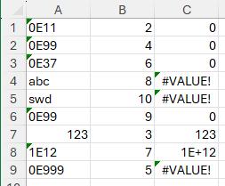
I believe "1E12" is converted to a number (not treated as text), but "0E999" is not because it exceeds Excel's numeric limit as explained by Tomek below.
One way to confirm this using the Tip's worksheet is to enter '1E12 in cell A8 and '0E999 in cell A9, then enter the following formula in cell C1
=1*A1
and drag that formula down to cell C9. The result (with cells formatted as General) is illustrated in (see Figure 1 below)

Figure 1.
2024-11-02 22:54:00
Tomek
Rather than modifying your original data, or using wild character match, you could create a helper column, say C in which you would convert the contents of the A column to something that is always a text. For example in cell C1 you could enter formula
=A1 & "n"
and copy it down for as many cells as needed. Then you could use a formula like
=SUMIF(C1:C7,"0E99n",B1:B7)
Another formula in the help column could be
=RIGHT(A1,3)
and then use
=SUMIF(C1:C7,"E99",B1:B7)
2024-11-02 22:24:35
Tomek
To understand this better, you have to realize that 0E99, 0E11, 0E37 or any 0EXX (each X being a digit) evaluates to 0 = 0 * 10^XX.
The same will happen for any 0EXXX as long as XXX is less than 308, as well as for any 0EX.
BTW, theoretically, the largest number that Excel can handle is 1.79769313486232E+308, but numbers with exponent 308 are handled inconsistently, often treated as text.
2024-11-02 07:26:35
Ruth Engle
Excell can run a filter down rows but I am wanting to run the same kind of filter across columns is there a way to do that without transposing the data or is there a way to filter rows and columns is what I would really like to do.
Got a version of Excel that uses the ribbon interface (Excel 2007 or later)? This site is for you! If you use an earlier version of Excel, visit our ExcelTips site focusing on the menu interface.
FREE SERVICE: Get tips like this every week in ExcelTips, a free productivity newsletter. Enter your address and click "Subscribe."
Copyright © 2026 Sharon Parq Associates, Inc.
Comments