SUM not Providing the Correct Sum

Bob has a simple formula that relies on the SUM function to total the 10 cells immediately above it. However, SUM doesn't seem to be returning the correct total. If Bob places 5 in each of the 10 cells, the SUM should be 50, but it only returns 35. Bob cannot figure out why he can't get the right sum with such a simple formula.

The first thing to check is that the SUM function is actually referencing all the cells in the range. You can easily figure this out by selecting the cell that contains the formula and then pressing F2. This puts Excel into edit mode, but it also highlights any cell ranges referenced within the formula. Make sure that the entire range of ten cells is highlighted. If it isn't, then adjust the formula to encompass the full range.

If the full range is being referenced, then the problem is probably related to the formatting of cells within the range. If some of the cells within the range are formatted as text—meaning, they were formatted as text before anything was in the cell—then they will be ignored by SUM, even if they contain a number.

This should be easy to figure out, though Excel's behavior can be a bit erratic. As an example, I placed, in cell H12, the following formula:

=SUM(H1:H10)

Then, I formatted cells H3, H6, and H8 as text. Next, starting in cell H1, I entered the value 5 in each cell, one cell at a time. I stopped before putting anything into cell H10. (See Figure 1.)

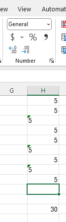
Figure 1. Entering data in the cells.

You can see that the three cells I formatted as text (H3, H6, and H8) are stored as left-justified text with the small, green corner triangle that lets you know there is something different about the cells. You can also see that I had entered 5 nine times, but the sum in H12 is 30, meaning that the SUM function recognized six numbers and three text values in the range. Finally, you can also see that cell H10 (the selected cell) is formatted as General.

Next, I typed 5 and pressed Enter. Then, I pressed the Up Arrow once to get back to cell H10. However, something funny had happened. (See Figure 2.)

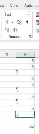
Figure 2. After entering cell H10.

Notice that the cell is now formatted as text and is left-justified, but there is no small, green corner triangle, and the value in cell H10 is included in the sum shown in cell H12—even though the cell is supposedly formatted as text!

When I entered the value in cell H10, Excel apparently noticed that cell H6 was formatted as text, cell H8 was formatted as text, and so to continue the every-other-cell pattern, it automatically formatted cell H10 as text.

This illustrates that Excel actually has two apparent ways to format a cell as text—either before entry or after entry. If I went back up to cell H4 and formatted it as text, with the value 5 already in there, then the value is left-justified, but the small, green triangle does not appear and the value is still included in the H12 sum. This is what happened with cell H10, which means that Excel considered that cell to be formatted as text post-entry, not pre-entry.

To make matters even messier, if I go back to one of my three cells that were formatted as text pre-entry (H3, H6, or H10), a small warning icon appears to the left of the cell. If I hover the mouse over that icon then I can click the down-arrow and see several different ways I can modify the cell contents. One of those options is "Convert to Number," which changes the cell formatting to General and makes the cell into a numeric value that is recognized by the SUM function.

It should be noted that this is the most efficient method of converting the text number into an actual number. If, instead, you simply format the cell using a numeric format (such as General), then Excel still treats the cell contents as text, even though the cell is not formatted as text. The solution at this point is to simply press F2 and Enter. This forces Excel to "re-parse" the cell contents and, since the cell uses a numeric format, it starts treating it as a number.

Another option in the icon drop-down list, though, is "Ignore Error." If you chose this option, then Excel gets rid of the small, green triangle and leaves the cell as text. At this point, the cell looks just like a numeric cell, but it is still left-justified. Of course, that justification could easily be changed by using the formatting tools on the Home tab of the ribbon, at which point it is much more difficult to tell that the cell is actually being treated as text.

This illustrates a very important concept—you cannot understand how Excel is interpreting a cell based solely on how the cell appears. You cannot even understand how Excel is interpreting the cell based on selecting the cell and looking at the Number Format drop-down list on the Home tab of the ribbon. If you really want to know how Excel is treating the cells, then you need to do the following:

1. Display the Excel Options dialog box. (In Excel 2007 click the Office button and then click Excel Options. In Excel 2010 or a later version, display the File tab of the ribbon and then click Options.)
2. At the left side of the dialog box, click Formulas. (See Figure 3.)



Figure 3. The Formulas area of the Excel Options dialog box.

3. Under the Error Checking heading, click the Reset Ignored Errors option.
4. Click OK to dismiss the Excel Options dialog box.

At this point, any cells containing numbers but that had been formatted as text pre-entry will display the small, green triangle. It is these cells that you need to pay attention to and convert to actual numbers instead of text.

ExcelTips is your source for cost-effective Microsoft Excel training. This tip (9632) applies to Microsoft Excel 2007, 2010, 2013, 2016, 2019, 2021, 2024, and Excel in Microsoft 365.