Conditionally Formatting an Entire Row

Graham described a problem he was having with a worksheet. He wanted to use conditional formatting to highlight all the cells in a row if the value in column E was greater than a particular value. He was having problems coming up with the proper way to do that.

Suppose for a moment that your data is in cells A3:H50. You can apply the proper conditional formatting by following these steps:

1. Select cell A3.
2. With A3 still selected, scroll the worksheet so you can see cell H50.
3. Hold down the Shift key as you click on H50. The entire range A3:H50 should be selected, and A3 should still be the active cell.
4. Make sure the Home tab of the ribbon is displayed.
5. Click the Conditional Formatting tool. Excel displays a series of choices.
6. Click New Rule. Excel displays the New Formatting Rule dialog box. (See Figure 1.)



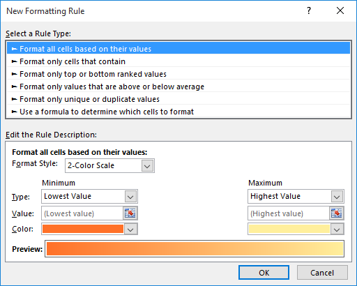
Figure 1. The New Formatting Rule dialog box.

7. In the Select a Rule Type area at the top of the dialog box, choose Use a Formula to Determine Which Cells to Format. (See Figure 2.)



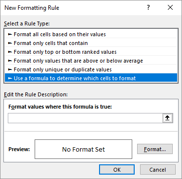
Figure 2. Use a Formula to Determine Which Cells to Format.

8. In the formula space, enter the following formula: =$E3>40000
9. Click the Format button. Excel displays the Format Cells dialog box. (See Figure 3.)



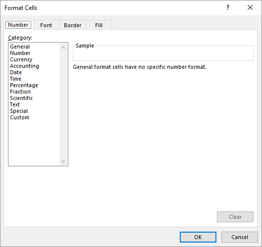
Figure 3. The Format Cells dialog box.

10. Using the controls in the dialog box, specify how you want the cells that are greater than 40,000 to be displayed.
11. Click OK to dismiss the Format Cells dialog box.
12. Click OK to accept your conditional format.

The formula used in the conditional format (step 8) works because you use the absolute indicator (the dollar sign) just before the column letter. Any reference that has the $ before it is not changed when Excel propagates it throughout a range. In this case, the cell reference will always be to column E, although the row portion of the reference can change.

ExcelTips is your source for cost-effective Microsoft Excel training. This tip (7360) applies to Microsoft Excel 2007, 2010, 2013, 2016, 2019, and Excel in Office 365. You can find a version of this tip for the older menu interface of Excel here: Conditionally Formatting an Entire Row.