Richard has a list of names and numbers (numeric values) in the range B1:B65. In cell A1 he has a single letter or a single digit. He would like to generate a list of just those values from B1:B65 that begin with the letter or digit in A1.
The thing that makes Richard's task a challenge is that both the contents of A1 and individual cells in B1:B65 can contain either text or numeric values. Even so, there are several ways you can approach this task. I'll focus first on using the newer Excel functions available in Excel 2021 and the version of Excel in Microsoft 365. If you are using one of these versions, you could use the following short formula:
=FILTER(B1:B65,LEFT(B1:B65,1)=""&A$1)
This works whether the value in A1 is text or numeric and whether the contents of B1:B65 are text or numeric; it doesn't matter. It works because of two interesting quirks of Excel. First, the LEFT function returns the leftmost character of whatever is in B1:B65 just fine, even if whatever is in B1:65 is numeric. And, because LEFT is a text function, it returns that character as text.
The second quirk is that ""&A$1 will return text because you are combining whatever is in A1 with "", which forces it to text. Thus, you end up comparing a text value coerced from column B with a text value coerced from cell A1. You could accomplish the same thing using this formula:
=FILTER(B1:B65,LEFT(B1:B65,1)=TEXT(A$1,0))
In this case, the TEXT function does the "forcing" to make sure that what is returned from cell A1 is text.
If you want to sort what is returned by the FILTER function, then you can wrap the formula in the SORT function:
=SORT(FILTER(B1:B65,LEFT(B1:B65,1)=""&A$1))
And, finally, if you think that the value in cell A1 might not be found in B1:B65, then you need to allow for that. The formulas so far will return a #CALC! error if this is the case. So, you can wrap your formula in an IFERROR function, in this way:
=IFERROR(SORT(FILTER(B1:B65,LEFT(B1:B65,1)=""&A$1)),"None")
This version of the formula returns your sorted list of matches, but if there are none, then it returns the text "None".
Again, these formulas discussed so far will work if you are using Excel 2021 or the version of Excel provided with Microsoft 365. If you are using an older version of Excel, then the easiest approach is to rely on a helper column. Enter the following into cell C1:
=IF(LEFT(B1,1)=""&$A$1,B1,"")
Copy this formula down to cells C2:C65 and you end up, in column C, with only those values from column B that begin with whatever is in cell A1. You can then copy these values to a different worksheet location and sort them, as desired, to have your list of cells that meet your criteria.
If you prefer a macro-based approach, you could use one similar to the following:
Sub CreateList()
    Dim J As Integer
    Dim K As Integer
    Dim sTemp As String

    sTemp = LCase(Left(Cells(1, 1).Text, 1))
    Range("D1:D65") = ""
    K = 0
    For J = 1 To 65
        If LCase(Left(Cells(J, 2).Text, 1)) = sTemp Then
            K = K + 1
            Cells(K, 4) = Cells(J, 2)
        End If
    Next J
End Sub
The macro places the matching cells into column D. If you would like the macro to be case sensitive, then simply remove the LCase function that appears two places in the macro. (None of the formulas presented earlier in this tip are case sensitive.) You would need to rerun the macro anytime you change values in either A1 or B1:B65.
Note:
ExcelTips is your source for cost-effective Microsoft Excel training. This tip (8308) applies to Microsoft Excel 2007, 2010, 2013, 2016, 2019, 2021, and Excel in Microsoft 365.

Dive Deep into Macros! Make Excel do things you thought were impossible, discover techniques you won't find anywhere else, and create powerful automated reports. Bill Jelen and Tracy Syrstad help you instantly visualize information to make it actionable. You�ll find step-by-step instructions, real-world case studies, and 50 workbooks packed with examples and solutions. Check out Microsoft Excel 2019 VBA and Macros today!
In mathematics, the sum of a range of sequential integers, starting with 1, is known as a triangular number or Gaussian ...
Discover MoreNeed to sum a series of cells that fits some regular pattern? Here are several ways that you can get the summation that ...
Discover MoreFor some operations and functions, Excel allows you to use wild card characters. One such character is an asterisk. What ...
Discover MoreFREE SERVICE: Get tips like this every week in ExcelTips, a free productivity newsletter. Enter your address and click "Subscribe."
2024-05-25 20:45:55
Tomek
One more note: If your data in the list changes, you will need to refresh the pivot table.
2024-05-25 20:32:04
Tomek
Part 3 was the last one, please read them starting from the one posted at 20:25:01 EDT
2024-05-25 20:28:25
Tomek
Part 3
You could explicitly enter the first character in the filter-cell F1, but I advise against it: you will get an error if such choice is not valid, but if you force it to be accepted that value will be remembered and mess up your available selections.
The only thing is, that your list will not be based on the content of the cell A1, but I hope this is acceptable. This is because you cannot use formula in the filter cell. You could create a macro that would put the value from the cell A1 into the filter cell F1, when a new value is entered in the cell A1, but I do not see a benefit for this, unless the value in the cell A1 is generated by other process, rather than entered manually.
Please note that the generated list of values shows unique values only. if a particular value exists twice or more times it will be shown only once. However, you could add the Count of List into the Σ Values area like I did - this will let you know how many times each value exists in your list.
Please also note that the listed values are not case sensitive.
2024-05-25 20:27:16
Tomek
Select all data in both columns (B and C) and click on Insert-Pivot Table. Confirm that your Table/Range covers all your data including the column headings. Select the location for the pivot table in an existing worksheet; in my demo it is the cell E1 in the same worksheet. (see Figure 1 below)
In the Pivot-Table-Fields pane ( see Figure 2 below) ), drag the FirstChar field to the filters area, and the List field to the Rows area. Now all you have to do is to click on the filter arrow and select from the list of available first characters. You can even select multiple filter values, if you check Select Multiple Items. (see Figure 3 below) .
For a cleaner look, remove row and column grand totals (in Pivot Table properties).
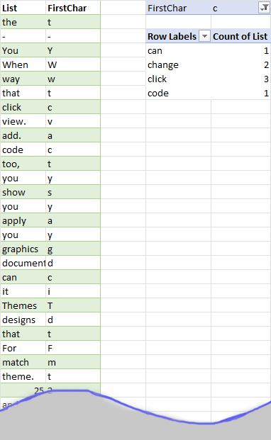
Figure 1.
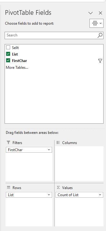
Figure 2.
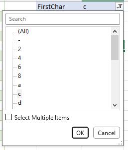
Figure 3.
2024-05-25 20:25:01
Tomek
I will post this in parts, because something in full post is triggering a rejection.
For earlier versions of Excel, I think an effective solution can be one based on a Pivot table used in a non standard way. It works with the newest versions too.
The data needs to be rearranged a little to allow for column headings, and a helper column, which will contain just the first character of each entry in the list. So, in the cell C2 enter:
=LEFT(B2,1)
Then copy this formula down for all the rows with data (doble-click on the small-square handle in the bottom-right of the cell, when the cell C2 is selected).
2024-05-25 19:06:39
Tomek
Re: And, finally, if you think that the value in cell A1 might not be found in B1:B65, then you need to allow for that. The formulas so far will return a
>#CALC! error if this is the case. So, you can wrap your formula in an IFERROR function, in this way:
>=IFERROR(SORT(FILTER(B1:B65,LEFT(B1:B65,1)=""&A$1)),"None")
----------------------------------------------------------
The FILTER function takes one more argument that specifies what to display if nothing is found:
=FILTER(B1:B65,LEFT(B1:B65,1)=""&A$1, "Not found")
This makes the use of IFERROR unnecessary
2024-05-25 16:24:07
J. Woolley
Here are two interesting points illustrated by this Tip:
1. As noted by Erik, the Tip's text comparison formulas ignore case, so an expression like
"A"="a"
is TRUE. For case-sensitive comparison of text, use
EXACT("A")=EXACT("a")
which is FALSE. For more on this subject, see https://excel.tips.net/T002165_Ignoring_Case_in_a_Comparison.html
2. Excel's TEXT(Value, Format_Text) function is supposed to require text like "@" for the Format_Text parameter, but the undocumented integer value 0 in the Tip's second formula seems to produce the same result as "@".
2a. Curiously, any numeric value for the Format_Text parameter is the same as "@" if the Value parameter is text or logical.
2b. But if the Value parameter is numeric and the Format_Text parameter is a non-zero integer, the function returns the Format_Text parameter.
2c. And if the Value and Format_Text parameters are both numeric but the latter is not an integer, the function returns the the Format_Text parameter combined with a rounded version of the Value parameter.
See (see Figure 1 below)
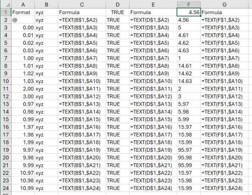
Figure 1.
2024-05-25 15:47:56
Erik
If you are planning to use helper cells, be aware that formula in the article above doesn't acknowledge any matches if A1 contains more than one character, even if the ID starts with the same multi-character value entered in A1.
The formula below uses only the first character in A1 even if more than one is entered by accident:
=IF( LEFT(B1,1) = LEFT($A$1,1), B1, "")
If you want to match more than one starting character, the following formula will count any ID that starts with whatever is in A1.
=IF( LEFT(B1,LEN($A$1)) = LEFT($A$1,LEN($A$1)), B1, "")
All three formulas handle numbers as text and ignore letter case (Abc = abc = ABC).
Got a version of Excel that uses the ribbon interface (Excel 2007 or later)? This site is for you! If you use an earlier version of Excel, visit our ExcelTips site focusing on the menu interface.
FREE SERVICE: Get tips like this every week in ExcelTips, a free productivity newsletter. Enter your address and click "Subscribe."
Copyright © 2026 Sharon Parq Associates, Inc.
Comments