Please Note: This article is written for users of the following Microsoft Excel versions: 2007, 2010, 2013, 2016, 2019, and 2021. If you are using an earlier version (Excel 2003 or earlier), this tip may not work for you. For a version of this tip written specifically for earlier versions of Excel, click here: Extracting URLs from Hyperlinks.
Mezga has a series of cells that contain hyperlinks. These hyperlinks consist of words such as "click here" or "more information." In other words, each hyperlink contains display text that is different from the underlying URL that is activated when the link is clicked. Mezga would like to know if there is a way, without using a macro, to extract the underlying URL for each of these hyperlinks and place that URL into a different cell.
Without using macros, you can do this:
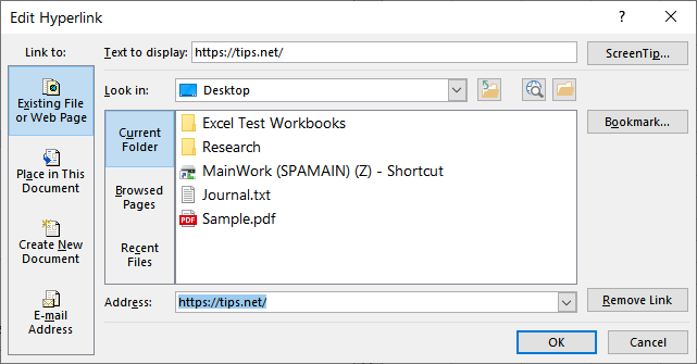
Figure 1. The Edit Hyperlink dialog box.
Note that this is for a single hyperlink. If you have a whole bunch of hyperlinks in a worksheet and you want to recover the URLs, you need to do this for each and every hyperlink. Obviously this can get tedious very quickly.
The cure for tedium—like them or not—is a macro. With a macro, getting at the underlying URL for a hyperlink is child's play. All the macro needs to do is pay attention to the Address property of the hyperlink. The following is an example of a macro that will find each hyperlink in a worksheet, extract each one's URL, and stick that URL in the cell directly to the right of the hyperlink.
Sub ExtractHL()
    Dim HL As Hyperlink
    For Each HL In ActiveSheet.Hyperlinks
        HL.Range.Offset(0, 1).Value = HL.Address
    Next
End Sub
Instead of a "brute force" macro, you could also create a user-defined function that would extract and return the URL for any hyperlink at which it was pointed:
Function GetURL(rng As Range) As String
    On Error Resume Next
    GetURL = rng.Hyperlinks(1).Address
End Function
In this case you can place it where you want. If you want, for example, the URL from a hyperlink in A1 to be listed in cell C25, then in cell C25 you would enter the following formula:
=GetURL(A1)
Note:
ExcelTips is your source for cost-effective Microsoft Excel training. This tip (9815) applies to Microsoft Excel 2007, 2010, 2013, 2016, 2019, and 2021. You can find a version of this tip for the older menu interface of Excel here: Extracting URLs from Hyperlinks.

Create Custom Apps with VBA! Discover how to extend the capabilities of Office 365 applications with VBA programming. Written in clear terms and understandable language, the book includes systematic tutorials and contains both intermediate and advanced content for experienced VB developers. Designed to be comprehensive, the book addresses not just one Office application, but the entire Office suite. Check out Mastering VBA for Microsoft Office 365 today!
When you add a hyperlink to a worksheet, over time and after doing a bunch of editing, what you see in the cell can get ...
Discover MoreIs your worksheet information destined for a Web page? Here's how you can specify the fonts that should be used when ...
Discover MoreYou can add hyperlinks to a worksheet and Excel helpfully makes them active so that when you click them the target of the ...
Discover MoreFREE SERVICE: Get tips like this every week in ExcelTips, a free productivity newsletter. Enter your address and click "Subscribe."
2026-04-01 11:01:23
Sandy T
To save some clicks, the shortcut to the Hyperlink dialog box is Ctrl-k.
Got a version of Excel that uses the ribbon interface (Excel 2007 or later)? This site is for you! If you use an earlier version of Excel, visit our ExcelTips site focusing on the menu interface.
FREE SERVICE: Get tips like this every week in ExcelTips, a free productivity newsletter. Enter your address and click "Subscribe."
Copyright © 2026 Sharon Parq Associates, Inc.
 Please Note:
This article is written for users of the following Microsoft Excel versions: 2007, 2010, 2013, 2016, 2019, and 2021. If you are using an earlier version (Excel 2003 or earlier), this tip may not work for you. For a version of this tip written specifically for earlier versions of Excel, click here:
Please Note:
This article is written for users of the following Microsoft Excel versions: 2007, 2010, 2013, 2016, 2019, and 2021. If you are using an earlier version (Excel 2003 or earlier), this tip may not work for you. For a version of this tip written specifically for earlier versions of Excel, click here:
Comments