Written by Allen Wyatt (last updated March 22, 2025)
This tip applies to Excel 2007, 2010, 2013, 2016, 2019, 2021, 2024, and Excel in Microsoft 365
Jose has a worksheet that has four comma-separated integers in column A, such as 5,6,9,13. These, obviously, are stored as text. There are hundreds of rows of values like this in the column. Jose wonders if there is a formula he can place in column B that will increment each integer, such as 6,7,10,14. He'd prefer to avoid separating the digits out to individual columns, if possible.
The answer to this depends largely on the version of Excel you are using. Or, I should say, the complexity of the answer depends on the version. If you want a formula that does not rely on functions in the newer versions of Excel, then you can use this in cell B1:
=LEFT(A1,FIND(",",A1)-1)+1 & "," &
MID(A1,FIND(",",A1)+1,FIND(",",A1,FIND(",",A1)+1)-FIND(",",A1)-1)+1 & "," &
MID(A1,FIND(",",A1,FIND(",",A1)+1)+1,FIND(",",A1,FIND(",",A1,FIND(",",A1)+1)+1)-FIND(",",A1,FIND(",",A1)+1)-1)+1 & "," &
RIGHT(A1,LEN(A1)-FIND(",",A1,FIND(",",A1,FIND(",",A1)+1)+1))+1
I've shown the formula here as four lines, but remember that it is all a single formula, entered on a single line. I broke it into four lines so it was more easily seen what it takes to increment the four numbers. (Each line is responsible for a single digit.) The FIND function is used to determine the location of each comma. The LEFT function is used to pull out the first number, the MID function the second and third numbers, and the RIGHT function the fourth numbers. Add 1 to each of the numbers forces Excel to treat the numbers as numeric values, and then the concatenation operator (&) forces the incremented numeric values back to text.
The drawback to the formula should be obvious—it is amazingly long. Plus, it will only work if there are four numbers separated by three commas. If there are more or less, then it will not work properly.
To get around these drawbacks, a macro-based solution was required. The following is an example of a macro that will easily pull apart any sequence of comma-separated values and return an incremented sequence:
Function IncrTxt(ByRef rng As Range, Optional iIncr As Integer)
    Dim var As Variant
    Dim str As String
    Dim i As Integer

    Application.Volatile
    If iIncr = 0 Then iIncr = 1
    var = Split(rng.Value, ",")
    For i = LBound(var) To UBound(var)
        str = str & var(i) + iIncr & ","
    Next i
    IncrTxt = Left(str, Len(str) - 1)
End Function
This is a user-defined function that can be placed into cell B1 in the following manner:
=IncrTxt(A1,1)
The second parameter is optional. It can be used if you want to increment the numbers by something other than 1.
Everything discussed so far will work in all versions of Excel. If you are using the latest versions, however, you have access to worksheet functions that can make the task a snap. Here's a simple formula you could use in B1 to do the job:
=TEXTJOIN(",",,TEXTSPLIT(A1,",")+1)
Then, copy the formula down for as many rows as necessary. The formula uses the TEXTSPLIT function to create an array of values by splitting the text string based on the commas. Each value is incremented by 1, and then TEXTJOIN is used to create a new string based on the incremented values separated by commas. This formula will only work for those using Excel 2024 or Microsoft 365 because those are the versions in which the TEXTSPLIT function is available.
Some may find this variation of the formula helpful:
=TEXTJOIN(",",,MAP(TEXTSPLIT(A1,","),LAMBDA(n,n+1)))
This formula relies on the MAP and LAMBDA functions to specify what should happen to each element of the array created by TEXTSPLIT. LAMBDA specifics that the value should be incremented by 1. To me, though, using MAP and LAMBDA for a simple increment seems to be a bit of overkill. It would be a more powerful approach, though, if Jose wanted something more complex done to each of the comma-separated numbers in column A. (The "more complex" concept will be illustrated in a moment in another use of LAMBDA.)
If you prefer to not use TEXTJOIN for some reason, you could instead use ARRAYTOTEXT, in this manner:
=ARRAYTOTEXT(TEXTSPLIT(A1,",")+1)
Note that ARRAYTOTEXT, in creating a new text string, automatically separates values by commas, while TEXTJOIN required the explicit specification of the delimiter to be used between values. The biggest difference, though, is that TEXTJOIN doesn't include a leading space for each number in the result whereas ARRAYTOTEXT does.
Note that these three formulas do not care how many comma-separated numbers are in the strings in column A. The formulas will work fine as long as there is at least one number in the cell in column A and if there are multiple numbers they are separated by only one comma. (In other words, the cell in column A cannot be blank and it cannot contain something like 5,6,,13 with two commas separating numbers.)
If you are absolutely sure that the strings in column A will always have four numbers separated by three commas, then you might want to consider this formula in cell B1:
=BYROW(TEXTSPLIT(TEXTJOIN("|",,A:A),",","|")+1,LAMBDA(row,TEXTJOIN(",",,row)))
This formula is more complex and therefore requires more explanation. It uses the first instance of TEXTJOIN to combine all the values in column A into a single string where each row is separated by a "|" character.
Using this super-long string of values, TEXTSPLIT is used to create a 4xN array of the numbers in column A. Each row in the array is defined by the "|" character. Essentially you end up with an array that is 4 columns by however many rows there are in column A. If any of the rows in column A are blank, then that row is ignored. Each of the values in the array created by TEXTSPLIT is then incremented by 1.
Finally, the BYROW function is used to apply a function to each row of the array returned by TEXTSPLIT. What function is it that is applied? In this case, the function is defined by the LAMBDA function which uses the second instance of TEXTJOIN to combine each of the 4 values in the array row being processed by BYROW. The BYROW function, after applying the LAMBDA function, returns a single row. Thus, each row spills over to a new worksheet row automatically.
This formula is much more complex than the earlier ones, but the benefit is that it processes everything in column A at once (you don't need to copy the formula downward) and it ignores any blank cells in column A.
Note:
ExcelTips is your source for cost-effective Microsoft Excel training. This tip (9950) applies to Microsoft Excel 2007, 2010, 2013, 2016, 2019, 2021, 2024, and Excel in Microsoft 365.

Dive Deep into Macros! Make Excel do things you thought were impossible, discover techniques you won't find anywhere else, and create powerful automated reports. Bill Jelen and Tracy Syrstad help you instantly visualize information to make it actionable. You�ll find step-by-step instructions, real-world case studies, and 50 workbooks packed with examples and solutions. Check out Microsoft Excel 2019 VBA and Macros today!
Averages and weighted averages are two related figures that must be approached differently from each other. This tip ...
Discover MoreIf you have a long numeric value in a cell, you may have a need to remove the last digit of that value. You can do so ...
Discover MoreWhen analyzing data, you may need to distill groupings from that data. This tip examines how you can use formulas and ...
Discover MoreFREE SERVICE: Get tips like this every week in ExcelTips, a free productivity newsletter. Enter your address and click "Subscribe."
2025-04-12 15:04:36
J. Woolley
@DuncanPT
Here's another way to document a cell's formula. Select the cell, then pick Formulas > Define Name (Alt+M+M+D) and give it a Name with Sheet scope, then describe the formula in the Comment box. See (see Figure 1 below)
My Excel Toolbox includes the following dynamic array function to list defined names with workbook, worksheet, or any scope, including names that are normally hidden:
=ListNames([Scope], [SkipHidden], [SkipHeader])
The list includes the following columns: Scope, Name, Visible, Refers To, Value, and Comment.
https://sites.google.com/view/MyExcelToolbox/
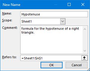
Figure 1.
2025-04-04 17:57:48
J. Woolley
@DuncanPT
You might be interested in My Excel Toolbox's ListFormulas function, which is described in my comment here: https://excelribbon.tips.net/T006198
You could use that function to list all of a target worksheet's formulas (or a selected range of formulas), then add your own description for each formula in the list.
https://sites.google.com/view/MyExcelToolbox/
2025-04-01 07:04:37
DuncanPT
@J.Woolley
Thanks that's very useful.
Although I have to say that as soon as it moves into T() vs N() and maneuvering around logical formulas, to me it shows as a workaround and not an MS thought-through feature. I would still have liked to see a proper comments layer, similar to but different from the Notes layer, but I suspect that is lost in history like the VHS/Betamax branch in the road...
2025-03-29 11:27:46
J. Woolley
@DuncanPT
See the following paragraph at https://excelribbon.tips.net/T011552
"There is another rather unique (and very esoteric) use for the N function—you can use it to add comments to formulas...."
Also, see my comment following that Tip.
2025-03-28 07:21:14
DuncanPT
A very interesting tip, with some new (to me) functions.
As a secondary issue, it also illustrates two / three problems with Excel:
1/ comments in formulas - I've always thought that Excel formulas rapidly become impossible to understand and I regret that there is no method of commenting or documenting them in a place associated with their cell. Even formatting them onto user-controlled multiple lines of logic as you did would be helpful.
2/ versions - unless you are sure of what version anyone using the spreadsheet will have, you have to go for the common denominator, ie simplest functionality approach. This dogged me in the middle of my career when my organisation, spread across 140 territories, had no single version of Excel in place and had to work at the most basic of levels to avoid long-distance help calls.
3/ new functions - related to 2/ above, I find that new functions appear out of the blue and unless you have a lot of training or familiarisation time available, yuou may never know they exist. I guess that is one of the point of value of Excel Tips!
2025-03-25 12:12:50
J. Woolley
My previous comments below cautioned, "The first argument of ForEachCell should be a limited range like A1:A99; don't try a complete column like A:A unless you have a lot of patience." My Excel Toolbox now includes a function to limit a target range based on a worksheet's used range. Here's an abbreviated version:
Function RangeUsed(Target As Range)
Set RangeUsed = Intersect(Target, Target.Worksheet.UsedRange)
End Function
A range (array of cells) is returned. The unabbreviated version includes options to return the address of Target's limited range or the worksheet's used range as text like [Book1.xlsx]Sheet1!$A1:$H$31.
A worksheet's used range is a rectangular region encompassing all cells that are not empty. Some cells within the used range might be empty, but all cells outside the used range are definitely empty. An empty cell is blank, but not all blank cells are empty. For example, a blank cell with a Number format that is not General is not empty unless its entire column or row has the same format.
Certain functions like ForEachCell and MAP can benefit by applying RangeUsed; for example:
=ForEachCell(RangeUsed(A:A), ...)
=MAP(RangeUsed(A:A), ...)
See https://sites.google.com/view/MyExcelToolbox
2025-03-22 14:30:21
J. Woolley
The Tip's final formula in cell B1 is
=BYROW(TEXTSPLIT(TEXTJOIN("|", , A:A), ",", "|") + 1,
LAMBDA(row, TEXTJOIN(",", , row)))
The result is an array in column B, but there are restrictions as described in my previous comment below. Here is a simpler formula with an array result in column B but without the same restrictions:
=MAP(A:A, LAMBDA(row, TEXTJOIN(",", , TEXTSPLIT(row, ",") + 1)))
This formula is similar to the ForEachCell(...) formula described in my previous comment; unfortunately both return #VALUE! for each blank row in column A. Here is one way to avoid that problem:
=MAP(A:A, LAMBDA(row, IF(row="", "",
TEXTJOIN(",", , TEXTSPLIT(row, ",") + 1))))
The equivalent My Excel Toolbox formula is
=ForEachCell(A1:A99, "IF(@="""", """",
JoinAsText("","", TRUE, SplitText(@, "","") + 1))")
Notice it is still important to limit the range of ForEachCell's first argument.
2025-03-22 11:45:24
J. Woolley
Several of the Tip's formulas use the following expression:
TEXTSPLIT(A1, ",") + 1
In this case a cell "cannot contain something like 5,6, ,13 with two commas separating numbers." Here is a substitute expression that does not have the same restriction:
REGEXEXTRACT(A1, "\d+", 1) + 1
In this case a number is represented by "\d+" (one or more digits), which can be separated from another number by any one or more non-digits. See
https://exceljet.net/formulas/split-text-string-to-character-array
The Tip's final formula is prefaced, "If you are absolutely sure that the strings in column A will always have four numbers separated by three commas...." The actual limitation is "...an equal quantity of numbers with each pair of numbers separated by a comma...."
My Excel Toolbox includes the following functions (which do not require Excel 2024 or Microsoft 365):
SplitText -- see my comment at https://excelribbon.tips.net/T009396
JoinAsText -- see my comment at https://excelribbon.tips.net/T009396
RegExMatch -- see my comment at https://excelribbon.tips.net/T009392
ForEachCell -- see my comment at https://excelribbon.tips.net/T011725
Therefore, the following formula in the Tip
=TEXTJOIN(",", , TEXTSPLIT(A1, ",") + 1)
can be replaced by
=JoinAsText(",", TRUE, SplitText(A1, ",") + 1)
An equivalent result is given by
=JoinAsText(",", TRUE, RegExMatch(A1, "\d+", 1) + 1)
And the Tip's final formula in cell B1
=BYROW(TEXTSPLIT(TEXTJOIN("|", , A:A), ",", "|") + 1,
LAMBDA(row, TEXTJOIN(",", , row)))
can be replaced by
=ForEachCell(A1:A99, "JoinAsText("","", TRUE, SplitText(@, "","") + 1)")
The latter formula assumes Jose's comma-separated integers are in the range A1:A99 and returns an array in B1:B99; a blank cell in A1:A99 will result in #VALUE! for the corresponding row in B1:B99. The first argument of ForEachCell should be a limited range like A1:A99; don't try a complete column like A:A unless you have a lot of patience. When using pre-2021 versions of Excel without support for dynamic arrays, review the PDF file UseSpillArray.pdf.
See https://sites.google.com/view/MyExcelToolbox
Got a version of Excel that uses the ribbon interface (Excel 2007 or later)? This site is for you! If you use an earlier version of Excel, visit our ExcelTips site focusing on the menu interface.
FREE SERVICE: Get tips like this every week in ExcelTips, a free productivity newsletter. Enter your address and click "Subscribe."
Copyright © 2026 Sharon Parq Associates, Inc.
Comments