Setting the Width for Row Labels

Lars has a worksheet that has a large amount of data—approximately 5,000 rows. At the top of the worksheet he has a graph based on that data, with the data itself starting at row 30. He has the top 30 rows frozen so that he can always see the graph and column headings. When he scrolls down through the data and gets to row 1000, the row labels (left side of screen) become wider and this forces Excel to redraw the graph. The redrawing slows down scrolling and would be unnecessary if Lars could find a way to set a width for the row labels, so they were wide enough to accommodate the four digits necessary for these "upper" rows.

There are a few ways you can approach this issue. The first is to simply turn off the row and column headings. To do so, follow these steps:

1. Display the Excel Options dialog box. (In Excel 2007 click the Office button and then click Excel Options. In Excel 2010 and later versions, display the File tab of the ribbon and then click Options.)
2. At the left of the dialog box click Advanced.
3. Scroll through the available options until you see the Display Options for this Worksheet section. (See Figure 1.)



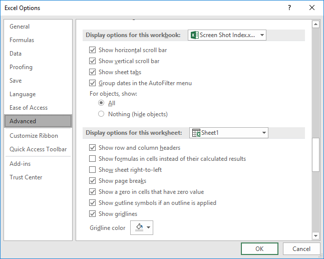
Figure 1. The Advanced options of the Excel Options dialog box.

4. Make sure the Show Row and Column Headers check box is selected. If cleared, then the header area is not displayed.
5. Click on OK.

Now you won't have the problem because Excel doesn't display the row headers at the left of the screen. If you really need to have some indication as to row number, you could always insert a blank column A, then insert numbers representing the row numbers, 1 through 5,000 (or however many rows there are). This column could be made as wide as necessary, so there won't be any redrawing as you scroll.

Another approach is to actually start your data and graph below row 1000. Insert enough blank rows above your graph and data to move them down into the four-digit row number range, and then hide rows 1 through 999.

A variant on this approach is to keep your graph where it is and insert enough rows to move just the data downward, so it starts at row 1000. Hide rows 30 through 999 and you should see no redrawing occur as you scroll.

ExcelTips is your source for cost-effective Microsoft Excel training. This tip (11677) applies to Microsoft Excel 2007, 2010, 2013, 2016, 2019, and Excel in Office 365. You can find a version of this tip for the older menu interface of Excel here: Setting the Width for Row Labels.