Written by Allen Wyatt (last updated January 11, 2025)
This tip applies to Excel 2007, 2010, 2013, 2016, 2019, 2021, 2024, and Excel in Microsoft 365
Roger is wondering if there is way to use the COUNTIF function using the cell background color as the "if" criteria. He has a calendar and he wants to be able to count the number of days he highlights in purple or other colors.
The short answer is that COUNTIF cannot be used to check for background color or any formatting; it can only test for values. If you only need to figure out the number of purple cells once or twice, you can use Excel's Find and Replace feature to figure it out. Follow these steps:
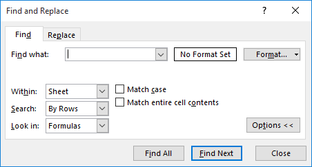
Figure 1. The Find tab of the Find and Replace dialog box.
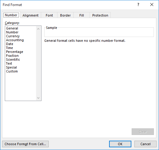
Figure 2. The Find Format dialog box.
Of course, these steps might get tedious if you want to count more than a color or two. Or, you may want the count so you can use it in a different calculation of some type. In these instances, you would do better to create a user-defined function that examines the cells and returns a count. One such macro is CountColorIf:
Function CountColorIf(rSample As Range, rArea As Range) As Long
    Dim rAreaCell As Range
    Dim lMatchColor As Long
    Dim lCounter As Long

    lMatchColor = rSample.Interior.Color
    For Each rAreaCell In rArea
        If rAreaCell.Interior.Color = lMatchColor Then
            lCounter = lCounter + 1
        End If
    Next rAreaCell
    CountColorIf = lCounter
End Function
In order to use the macro, all you need to do is provide a cell that has the background color you want tested and the range to be tested. For instance, let's say that cell A57 is formatted with the same purple background color you use in your calendar cells. If the calendar is located in cells A1:G6, then you could use the following to get the count of purple cells:
=CountColorIf(A57, A1:G6)
It should be noted that if you change the color in a cell in your calendar, then you'll need to do something to force a recalculation of the worksheet. It seems that Excel doesn't do an automatic recalculation after changing background color.
There are, of course, many different ways you could approach the problem and develop user-defined functions such as CountColorIf. Here are a couple other websites that contain information that may be helpful in this regard:
http://www.cpearson.com/excel/colors.aspx
https://www.ozgrid.com/VBA/sum-count-cells-by-color.htm
There are also some third-party add-ons available that you could use. One such add-on suggested by readers is Kutools for Excel. You can find more information on the add-on here:
https://www.extendoffice.com/product/kutools-for-excel.html
One final note—the ideas in this tip work fine if you are working with cells that are explicitly filled with colors. They will not work with cells that are colored using Conditional Formatting. That is an entirely different kettle to boil, as Conditional Formatting doesn't really give you anything you can latch onto easily.
Note:
ExcelTips is your source for cost-effective Microsoft Excel training. This tip (11725) applies to Microsoft Excel 2007, 2010, 2013, 2016, 2019, 2021, 2024, and Excel in Microsoft 365.

Best-Selling VBA Tutorial for Beginners Take your Excel knowledge to the next level. With a little background in VBA programming, you can go well beyond basic spreadsheets and functions. Use macros to reduce errors, save time, and integrate with other Microsoft applications. Fully updated for the latest version of Office 365. Check out Microsoft 365 Excel VBA Programming For Dummies today!
In the newest version of Excel, a change in how formulas are calculated can cause havoc for some "older" formulas. Here ...
Discover MoreWant to return more than a value when doing a lookup? Here are a couple of ways to do it by adding an IF clause to your ...
Discover MoreIf you need to know the number of columns in a particular range, you can use the COLUMNS worksheet function. This tip ...
Discover MoreFREE SERVICE: Get tips like this every week in ExcelTips, a free productivity newsletter. Enter your address and click "Subscribe."
2025-04-08 18:27:08
J. Woolley
My most recent comment below described COUNTIF2, COUNTIFS2, SUMIF2, and SUMIFS2, which work with arrays as well as ranges; the corresponding Excel functions only work with ranges. Mea culpa; the original implementation of COUNTIFS2 and SUMIFS2 was incorrect, but the latest version has resolved the problem. In addition, the following functions have been introduced to complement corresponding Excel functions and work with arrays as well as ranges: AVERAGEIF2, AVERAGEIFS2, MAXIF2, MAXIFS2, MINIF2, and MINIFS2.
See https://sites.google.com/view/MyExcelToolbox/
2025-02-04 10:38:54
J. Woolley
My comment dated 2025-01-20 below describes the ForEachItem and ForEachCell functions in My Excel Toolbox. It suggests the following formula to count the number of cells in the range A2:A25 having a fill color that matches cell A8:
=SUM(--(ForEachItem(A2:A25, "FillColor(@)") = FillColor(A8)))
That formula sums the double unary of logical results.
The following formula might seem more appropriate
=COUNTIF(ForEachItem(A2:A25, "FillColor(@)"), FillColor(A8))
but it fails because Excel's COUNTIF function only accepts a range of cells as its first argument (like Tomek's helper column range B2:B25), not the array of values returned by ForEachItem.
The following Excel functions only accept cell ranges: COUNTIF, COUNTIFS, SUMIF, and SUMIFS. My Excel Toolbox now includes COUNTIF2, COUNTIFS2, SUMIF2, and SUMIFS2; these alternate versions work with arrays as well as ranges. Therefore, the following formula returns the number of cells in Tomek's Figure 1 that have a fill color matching cell A8:
=COUNTIF2(ForEachCell(A2:A25, "FillColor(@)"), FillColor(A8))
With this formula the helper column in B is unnecessary.
See https://sites.google.com/view/MyExcelToolbox/
2025-01-26 15:19:13
J. Woolley
My earliest comment below described the FillColor function to return the base RGB fill color of a cell as a decimal value. That function has been modified to return "conditional" if the cell has a conditional format specifying a fill color different from the base, even if the condition is not satisfied. Here is an abbreviated version:
Function FillColor(Cell As Range)
FillColor = Cell.Interior.Color
Dim FC As FormatCondition
For Each FC In Cell.FormatConditions
With FC.Interior
If Not (.ColorIndex = xlColorIndexNone Or IsNull(.ColorIndex)) Then
If .Color <> FillColor Then FillColor = "conditional": Exit For
End If
End With
Next FC
End Function
See https://sites.google.com/view/MyExcelToolbox/
2025-01-22 18:33:22
Tomek
@ sandeep
The limitation is that the suntax
<cell>.DisplayFormat.Interior.Color
cannot be used within user defined function UDF) see https://learn.microsoft.com/en-us/office/vba/api/excel.range.displayformat
However the following will work:
==============
Public Sub GetDisplayedColors()
'populate cells K columns to the right of the selection
' with color displayed in the cells in the selection.
'The color may be from conditional or explicit formatting.
Dim cl As Range, K As Integer
K = 1
'un-comment the next line if you want the user to specify offset.
'K = InputBox("Offset?", "Enter number of columns.", K)
For Each cl In Selection
cl.Offset(0, K).Value = cl.DisplayFormat.Interior.Color
Next
End Sub
===============================
You just need to select the range of cells for which you want to get the displayed colors, then run the Sub. The RGB value for the color of each cell in the selection will be placed K cells to the right. It will use conditional color if it is applied. If you have a calendar with several columns you can increase the value of K and uncomment the line as indicated above, so that the RGB values do not overlap your original data, otherwise the values are put in the next cell to the right.
2025-01-21 04:12:35
sandeep
Dear Tomek, Please enlighten me how to overcome the limitation.
2025-01-20 10:14:23
J. Woolley
Certain functions in Excel and My Excel Toolbox accept a single value but not an array or multi-cell range. Often it is necessary to create a helper column with the function in a column of cell formulas; first enter a formula at the head of the column, then copy the formula down the remainder of the column.
My most recent comment below discusses Excel 365's MAP function to create a virtual helper column as an array. The following function in My Excel Toolbox is similar to MAP:
=ForEachItem(Items, Formula)
This function evaluates a Formula for each item in Items. The results are returned in an array matching the dimensions of Items, which can be a single value, an array of values (1D or 2D), or a range of cells. Formula must be the text equivalent of a cell formula using @ to represent one item in Items. Formula can begin with or without an equal sign, so "=SIN(@)" and "SIN(@)" are equivalent. Each item in Items will replace all instances of @ before Formula is evaluated for that item. You can use @ to escape @; i.e., @@ will be replaced by @ as text, not by an item in Items.
If Items is a range of cells, ForEachItem returns results from the following My Excel Toolbox function (with Items replacing Target):
=ForEachCell(Target, Formula)
Target must be a range of cells. Only its first contiguous area applies; any other areas are ignored. For example, if Target is (A1:C3, D1, E1:F2), which has three areas, only A1:C3 applies. Formula is the same as before.
For example, if the value of A3 is 10, A4 is 20, B3 is abc, and B4 is xyz, then this formula
=ForEachCell(A3:B4, "@ & ""@@"" & CELL(""address"", @)")
returns the following 2x2 array of text values:
{ 10@$A$3, abc@$B$3; 20@$A$4, xyz@$B$4 }
Notice when Formula is a quoted string, any quotation marks within the string must be doubled. This could be avoided if cell E3 contained the following text constant:
@ & "@@" & CELL("address", @)
In this case, the previous formula could be replaced by
=ForEachCell(A3:B4, E3)
The last formula in my most recent comment below was
=SUM(--(MAP(A2:A25, LAMBDA(x, FillColor(x))) = FillColor(A8)))
Using ForEachItem instead of MAP, the following formula returns the same result:
=SUM(--(ForEachItem(A2:A25, "FillColor(@)") = FillColor(A8)))
Notice ForEachItem could be replaced by ForEachCell because A2:A25 is a range of cells, not an array of values.
See https://sites.google.com/view/MyExcelToolbox/
2025-01-18 15:33:46
J. Woolley
Tomek's approach was to create a helper column in B with each cell containing the decimal RGB value of the fill color for the corresponding cell in column A, then use COUNTIF to count column B values that match the RGB value of a specified color. This is a typical solution method because his ClColor function can only return the fill color for a single cell. If it could return an array containing the fill color for each cell in a range of cells, then the helper column would not be necessary; in that case, this formula would count the number of cells with the same violet color as cell A8 (see Figure 1 in Tomek's first comment below):
=SUM(--(ClColor(A2:A25) = ClColor(A8)))
Notice the following formula would fail because COUNTIF requires its first argument to be a range and will not accept an array even if ClColor could return one:
=COUNTIF(ClColor(A2:A25), ClColor(A8)) -- returns #VALUE!
Excel 365 includes the MAP function, which offers another method to avoid the helper column. Here is the solution using MAP:
=SUM(--(MAP(A2:A25, LAMBDA(x, ClColor(x))) = ClColor(A8)))
The MAP(A2:A25, LAMBDA(...)) function above replaces x by each cell in the range A2:A25, returning the desired array of ClColor results.
As described in my previous comment below, My Excel Toolbox's FillColor function can be substituted for Tomek's ClColor function in this discussion. So this formula returns the same result:
=SUM(--(MAP(A2:A25, LAMBDA(x, FillColor(x))) = FillColor(A8)))
By the way, MAP will accept either a range or an array for its first argument.
2025-01-12 12:06:03
J. Woolley
My Excel Toolbox includes the following function to return the RGB fill color of a cell as a decimal value:
=FillColor([Cell])
The default value of Cell is the formula's cell. If Cell is a multi-cell range, only its first cell applies. This function is essentially the same as the ClColor function described in Tomek's earliest comment below; it ignores conditional formatting.
My Excel Toolbox also includes the following function to convert a decimal RGB color value into a 6-character hexadecimal text value:
=ColorAsHex(ColorRGB)
For example, the decimal RGB value for red is 255; its hexadecimal text value is FF0000.
To return the RGB fill color of a cell as hexadecimal text, use this formula:
=ColorAsHex(FillColor([Cell]))
See https://sites.google.com/view/MyExcelToolbox/
For more about colors, see my earliest comment (2024-07-05) here: https://excelribbon.tips.net/T009092_Showing_RGB_Colors_in_a_Cell.html
2025-01-11 19:08:26
Note to the picture in my previous comment:
The Figure 1 shows 5 violet cells found, but if you count the colors you will only find 4. That is because the cell A12 has conditional formatting applied to it with yellow background and it takes precedence when displayed. The explicit background color is still 15086320 as indicated in B12.
I just forgot remove conditional formatting, but it proves the point that this approach does not necessarily reflect what you see.
I actually suspect that Roger would like to count the cells by color that is defined by conditional formatting. Contrary to what Allen said, this information can be obtained by VBA by using the following syntax:
<cell>.DisplayFormat.Interior.Color
It will get the color of what is displayed, whether it is explicit, or overridden by conditional formatting.
Unluckily this syntax cannot be used in user defined functions, but can be used in subs.
I have some ideas how to overcome this limitation, so if someone is interested please reply here or send me an e-mail.
2025-01-11 17:10:58
Tomek
A different approach would be to create an user defined function that would return a color of the cell background, e.g,:
'===============================================
Public Function ClColor(cl As Range)
ClColor = cl.Interior.Color
End Function
'==============================================
Then you can create a mirror range of cells containing the color values for the range of cells in the calendar, using a formula =ClColor(address) (see Figure 1 below) .
Let's assume this range is named "CalendarShades"
Then in a cell where you want the count enter:
=COUNTIFS(CalendarShades,15086320))
where the number 15086320 corresponds to violet color of the cell background in the example spreadsheet.
Note that the range of cells does not have to be contiguous or rectangular.
I suggest creating the mirror range on a second sheet, simply by creating the duplicate sheet, then replacing the content of the relevant cells with the formula for the color from original sheet.
Like it was stated in Allen's tip, this approach will also work only with cells that are explicitly filled with colors.
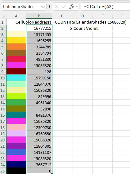
Figure 1.
Got a version of Excel that uses the ribbon interface (Excel 2007 or later)? This site is for you! If you use an earlier version of Excel, visit our ExcelTips site focusing on the menu interface.
FREE SERVICE: Get tips like this every week in ExcelTips, a free productivity newsletter. Enter your address and click "Subscribe."
Copyright © 2026 Sharon Parq Associates, Inc.
Comments