Sorting Dates by Month

There may come a time when you have a need to sort a list of information based on the month represented in a particular column. For instance, you may have a list of people and their birthdays, and you want to sort the list by birthday month so that you know whose birthdays occur within a particular month.

The easiest way to do this is to add a new column to your table. This column will be named something descriptive, such as "Birth Month" or simply "Month." For instance, let's say that you have people's birthdays in column B, you could add the new column in column C. In this column you could then use the MONTH function, as follows:

=MONTH(B3)

This particular formula would go in cell C3, but similar formulas would go in each cell of column C. The result is that column C will contain numbers ranging between 1 and 12, representing to birth months of the people. You can now sort the list based on the contents of column C, with the result that the list is sorted by month.

This approach works fine, but you may not be able to add another column to your worksheet. If this is the case, you can follow these steps to sort by month:

1. Select the cells in column B (assuming that column B contains the birthdates).
2. Press Ctrl+Shift+F. Excel displays the Format Cells dialog box.
3. Make sure the Number tab is displayed.
4. In the Category list, choose Custom. (See Figure 1.)



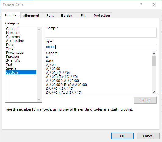
Figure 1. The Number tab of the Format Cells dialog box.

5. In the Type box, enter four lowercase Ms (mmmm) for the format.
6. Click on OK. The cells in column B should now show only the birth month of the people in your list. (Don't worry; the underlying birthdates are still there.)
7. Select your entire list.
8. Display the Data tab of the ribbon.
9. Click Sort in the Sort & Filter group. Excel displays the Sort dialog box. (See Figure 2.)



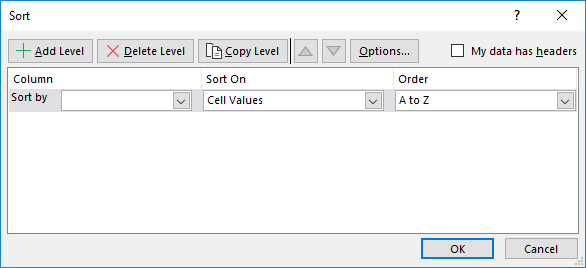
Figure 2. The Sort dialog box.

10. Use the controls in the dialog box to specify that you want to sort by the contents of column B.
11. Use the Order drop-down list to choose Custom List. Excel displays the Custom List dialog box.
12. From the available custom lists, select the one that lists months and then click OK.
13. Click on OK to close the Sort dialog box and actually sort the list.

You may be wondering why you need to reformat the display of the cells containing the birthdates (steps 1 through 6). The reason is that when you finally sort your list (steps 7 through 13), if you simply have the original full dates displayed, Excel will effectively sort the list chronologically rather than by month.

There is an additional way you can approach the problem. This involves actually converting the dates into text (instead of the internal serial numbers), as follows:

1. Select the cells that contain the dates.
2. Press Ctrl+Shift+F. Excel displays the Format Cells dialog box.
3. Make sure the Number tab is selected.
4. In the list of Categories, choose Date.
5. In the list of Types, choose March 14, 2012.
6. Click on OK. Your cells should now be formatted to show a long date with the month first.
7. Press Ctrl+C. This copies the cells to the Clipboard.
8. Open Notepad.
9. Press Ctrl+V. The information is now pasted into Notepad, and should still be the long dates.
10. Select the information just pasted into Notepad.
11. Press Ctrl+C. This copies the information to the Clipboard.
12. Switch back to Excel.
13. Press Ctrl+Shift+F. Excel displays the Format Cells dialog box.
14. Make sure the Number tab is selected.
15. In the list of Categories, choose Text.
16. Click on OK.
17. Press Ctrl+V.

Your dates are now pasted into Excel as true text entries, not as dates. This allows you to easily sort the information according to the month in the date.

ExcelTips is your source for cost-effective Microsoft Excel training. This tip (9728) applies to Microsoft Excel 2007, 2010, 2013, 2016, 2019, and 2021. You can find a version of this tip for the older menu interface of Excel here: Sorting Dates by Month.