Creating Two-Line Custom Formats

Excel is quite flexible in how it allows you to set up custom formats for displaying all sorts of values. Most custom formats are straightforward and easy to figure out, once you understand how custom formats work. (Custom formats and how to set them up has been discussed fully in other issues of ExcelTips.)

What if you want to create a two-line custom format, however? For instance, you may want to format a date so that the abbreviated day of the week and day of the month is on the first line, followed by the unabbreviated name of the month on the second line. Using such a format, a date would appear in a single cell in this manner:

Sat 13
April

Most of this can be done by the custom format "ddd d mmmm", but you need to figure out a way to add a line break between the "d" and the "mmmm". Excel won't let you press Alt+Enter between them, which is what you normally do to add a line break.

The solution is to use the numeric keypad to enter the desired line break in the format. Follow these steps to set it up:

1. Select the cells you want to format.
2. Display the Home tab of the ribbon.
3. Click the small icon at the bottom-right of the Number group. Excel displays the Number tab of the Format Cells dialog box.
4. In the Category list, choose Custom. (See Figure 1.)



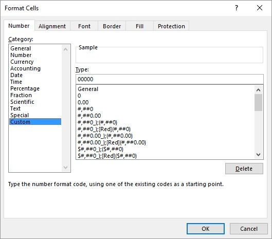
Figure 1. The Number tab of the Format Cells dialog box.

5. Delete whatever is in the Type box.
6. Type "ddd d" without the quote marks.
7. Either press Ctrl+J or hold down the Alt key while you press 0010 on the numeric keypad. This enters the line feed character, and it looks like the portion of the format you typed in step 6 disappears. It is not really gone; the insertion point has simply moved to a position you can't easily see. Watch the Sample area in the dialog box to verify the format as you continue typing.
8. Type "mmmm" without the quote marks.
9. Click the Alignment tab. (See Figure 2.)



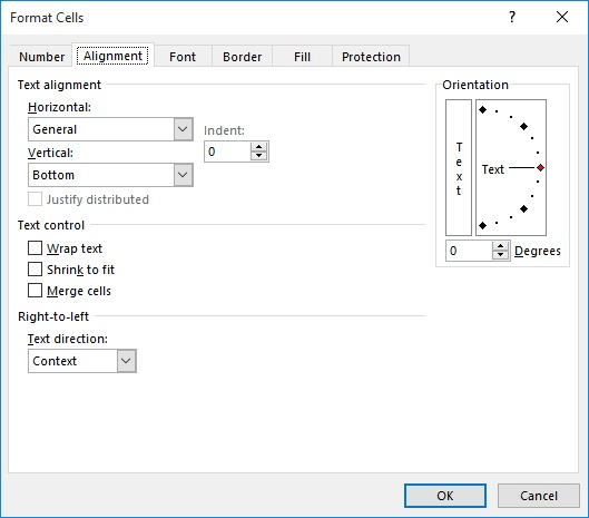
Figure 2. The Alignment tab of the Format Cells dialog box.

10. Make sure the Wrap Text check box is selected.
11. Click OK.

After setting up the format in this manner, you will need to adjust the row height of the formatted cells so that the entire two lines of the date will display.

You may also need to adjust the column width. Even though the display is on two lines, Excel may calculate column width as if the formatted value were on one line; if the column is too narrow you may see #####. One thing to try is to use the Alignment options in the Format Cells dialog box: turn Wrap Text off, turn on Shrink to Fit, and then turn Wrap Text back on. Depending on your data, you may also find that centering the cell content horizontally makes the extra whitespace less noticeable.

ExcelTips is your source for cost-effective Microsoft Excel training. This tip (12587) applies to Microsoft Excel 2007, 2010, 2013, 2016, 2019, 2021, 2024, and Excel in Microsoft 365. You can find a version of this tip for the older menu interface of Excel here: Creating Two-Line Custom Formats.