Written by Allen Wyatt (last updated March 16, 2024)
This tip applies to Excel 2007, 2010, 2013, 2016, 2019, 2021, and Excel in Microsoft 365
Hazel does a lot of manual entry into a worksheet, and any numbers she places into rows 10 through 120 need to be negative. She wonders if there is a way to enter values in these rows as negatives without the need to type the minus sign for each one.
Theoretically this is rather easy to do. All you need to do is to select the cells (in this case, rows 10:120) and then apply a custom format similar to this: -#,##0.00
Now, whenever you enter a positive value into any of the cells, it will show up as negative. This, despite the fact that the underlying number is actually positive. If you use these values in any formulas, they will show as negative as long as the cell with the formula utilizes the same custom format.
Of course, this could lead to some weird results that you may not want. For instance, the square of a negative value is always a positive value, but if you square the value in a cell formatted with the custom format and then use the same custom format for the result, you get a negative result. As an example, say cell A12 contains the value 4. The custom format makes it appear as -4, and then if you use the formula =A12*A12 in cell B3, if you format B3 with the same custom format, then the result shown there will be -16.
Perhaps a better approach is to simply enter the values as regular, non-negative values and, after you are done, perform the following steps:
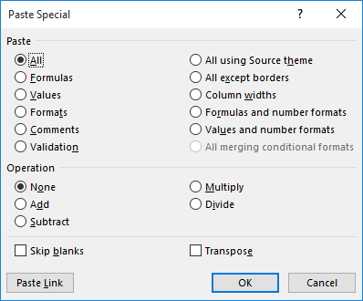
Figure 1. The Paste Special dialog box.
At this point Excel multiplies the values in the selected cells by the value in the Clipboard. Of course, if you now enter any new values into the target range, you will need to enter them as negatives. If you, instead, try to do the above steps again, then any existing negative values will become positive and any positive values will become negative.
Another approach is to utilize an event handler to do the proper conversion. The following is an example that could be used. (Right-click the worksheet's tab and choose View Code from the resulting Context menu.)
Private Sub Worksheet_Change(ByVal Target As Range)
    On Error GoTo ErrExit
    If Target.Row >= 10 And Target.Row <= 120 Then
        If Target.Value > 0 Then Target.Value = -Target.Value
    End If
ErrExit:
    Application.EnableEvents = True
End Sub
The event handler is quite simple in concept—it checks to see if a change is being made in the rows 10:120. If so, and the value in the cell is more than 0, then it is negated. You could also opt to use a more robust version that allows for the checking of multiple cells in the range:
Private Sub Worksheet_Change(ByVal Target As Range)
    Dim targ As Range, cell As Range
    Set targ = Application.Intersect(Target, Me.Range("10:120"))
    If targ Is Not Nothing Then
        Application.EnableEvents = False
        On Error GoTo ErrExit
        For Each cell In targ.Cells
            On Error GoTo ErrExit
            If IsNumeric(cell) And _
              Not (cell <= 0 Or IsDate(cell) Or cell.HasFormula) _
              Then cell = -cell '.Value is default property
ErrExit:
        Next cell
    Application.EnableEvents = True
End Sub
Note:
ExcelTips is your source for cost-effective Microsoft Excel training. This tip (13117) applies to Microsoft Excel 2007, 2010, 2013, 2016, 2019, 2021, and Excel in Microsoft 365.

Dive Deep into Macros! Make Excel do things you thought were impossible, discover techniques you won't find anywhere else, and create powerful automated reports. Bill Jelen and Tracy Syrstad help you instantly visualize information to make it actionable. You�ll find step-by-step instructions, real-world case studies, and 50 workbooks packed with examples and solutions. Check out Microsoft Excel 2019 VBA and Macros today!
Few things are as frustrating as trying to delete rows or columns and having Excel tell you that you can't perform the ...
Discover MorePaste information in a worksheet, and you may end up with Excel placing it into lots of different cells. If you want it ...
Discover MoreHow successful you are in copying information in Excel depends on lots of issues. This tip examines how those issues can ...
Discover MoreFREE SERVICE: Get tips like this every week in ExcelTips, a free productivity newsletter. Enter your address and click "Subscribe."
2024-03-18 17:33:17
Tomek
@Hazel Kohler,
If you use Ron S's suggestion of the helper column, I would put the input cells on a separate sheet, rather that having a helper column to hide and unhide. That way you can switch to the other sheet when entering the negative data and do everything else on the main sheet, which may be a visual hint to indicate when you are entering numbers to be negative. You can even protect the range in question on the main sheet from entering data there, with a pop up message directing you to input cells. Going overboard, you can also allow entry of only positive numbers on the helper sheet, and only in specified rows (10 to 120).
This may seem as too much work,if you are the only one who uses that workbook, but may be worthwhile if there may be other users that need to enter such data.
The formula to use on main sheet would be something like for cell B10:
=-InputSheet!B10
2024-03-18 17:32:00
Tomek
@Hazel Kohler,
It is nice to see that the person requesting help actually reads and appreciates the answer.
And, no, I did not contribute to this tip (yet), so I am saying this without personal interest.
2024-03-16 18:34:54
Ron S
You will need to use a "helper column".
Column A, enter values
Column B in rows 10-120 enter formula =Abs(B2)*-1
Column B rows 120+ enter formula =b2
This page lists several other methods including a chart listing pro's and cons for each method:
https://www.upwork.com/resources/how-to-make-numbers-negative-in-excel
Still with helper column A, end value col B, single formula:
=IF(ROW()<121, A10*-1, A10)
Copy the formula down to row 120
If you want to hide the input row, AND you do data entry at different times you could use PowerQuery.
Define your input area as an Excel Table, no helper column
Use PQ to read that input table
In PQ create a step to apply the formula (from above) in helper column
Next step delete the input column
Do any other data cleanup, or even formulas you need
Output to a new table on a new tab
Now you have 2 tabs:
one for input only
the other for user viewing of the output, without formulas.
After that the process is simple, do your data entry in the entry tab
then swap to the output tab, select the output table and use the "Refresh" function to import and process new data to update the output table.
https://support.microsoft.com/en-gb/office/refresh-an-external-data-connection-in-excel-1524175f-777a-48fc-8fc7-c8514b984440
I'm a strong fan of PowerQuery when data entry is required more than once. PowerQuery can be used to hide formulas from the users.
PowerQuery output is also a great input for Pivot Tables to generate summary reports!
PowerQuery and PivotTables take some time to learn, but once you get past the fear and invest some time for DYI learning (or pay for some courses) the combination can be used to save you days of repetitive work each week/month by automating collection of data from one or more sources and creating automated reports that just need a refresh to import new data.
PivotTables will impress your boss. Especially at how quickly you can tweak them to create new reports. If your boss is not willing to pay for the courses, any time you save by learning the skill you can use to surf the web or play solitaire on your phone (not your work computer! bosses can spy on them!)
2024-03-16 17:09:56
J. Woolley
In the Tip's first Worksheet_Change event procedure, Target.Value generates an error when negated if it is text or is formatted as Date (but not Time); in this case Target.Value is not changed. If Target.Value is TRUE (-1 in VBA) or FALSE (0 in VBA) it is not changed because it is not > 0. But if Target.Value is a positive numeric value the event procedure is triggered twice because EnableEvents was not disabled; in this case, if Target contains a formula it is replaced by a negative constant. The same applies to Micky's version, since Value is the default property of Target (a Range object).
If a multi-cell range is selected (contiguous or not) and a value is manually entered, the event procedure applies only to the active cell (Target is that single cell). But if a value is pasted into a multi-cell selection, then Target is that selection and the results depend on whether or not it is contiguous; when it is not contiguous (more than one area), the results depend on its configuration.
To resolve these issues, here is my version of the Tip's first event procedure:
Private Sub Worksheet_Change(ByVal Target As Range)
If Target.Row < 10 Or Target.Row > 120 Then
Exit Sub
ElseIf Not IsNumeric(Target.Value) Then
Exit Sub
ElseIf Target.HasFormula Then
Exit Sub
ElseIf Target.Value > 0 Then
Application.EnableEvents = False
Target.Value = -Target.Value
Application.EnableEvents = True
End If
End Sub
Notice IsNumeric(Target.Value) returns False if Target.Value is text or formatted as Date (but not Time); in this case Target.Value is not changed. And if Target contains a formula it is not disturbed. But when Target is a single cell with a positive numeric value the event procedure is triggered only once because EnableEvents is disabled before Target.Value is negated.
As before, if a multi-cell range is selected (contiguous or not) and a value is manually entered, the event procedure applies only to the active cell. When pasting into a contiguous multi-cell selection, IsNumeric(Target.Value) returns False and Target.Value is not negated. But if a value is pasted into a non-contiguous selection (more than one area), the results depend on its configuration.
To resolve issues with pasting into multiple cells, here is my version of the Tip's second event procedure:
Private Sub Worksheet_Change(ByVal Target As Range)
Dim targ As Range, cell As Range
Set targ = Application.Intersect(Target, Me.Range("10:120"))
If targ Is Nothing Then Exit Sub
For Each cell In targ.Cells
If IsNumeric(cell) And Not cell.HasFormula Then
If cell > 0 Then
Application.EnableEvents = False
cell = -cell '.Value is default property
Application.EnableEvents = True
End If
End If
Next cell
End Sub
This version is recommended for Hazel. It must be located in the applicable Sheet module as noted in the Tip: "Right-click the worksheet's tab and choose View Code from the resulting Context menu."
2024-03-16 16:52:35
Hazel Kohler
Thank you to everyone who helped on this question. It will save me a lot of time and key strokes
2024-03-16 07:49:46
MICHAEL (Micky) AVIDAN
To my opinion, due to limiting the bench of rows - there in no need to use any ENABLEEVENT command.
The following code should do the job.
Private Sub Worksheet_Change(ByVal Target As Range)
On Error GoTo ErrHandler
If Not Intersect(Target, Rows("10:120")) Is Nothing And Target > 0 Then Target = -Target
ErrHandler:
End Sub
2024-03-16 05:37:25
Joël Courtheyn
The last macro did not work for me, I have made two modifications : changed the location of the Not on line 4 and included and End if after Next cell as indicated in the revised code below
Private Sub Worksheet_Change(ByVal Target As Range)
Dim targ As Range, cell As Range
Set targ = Application.Intersect(Target, Me.Range("10:120"))
If Not targ Is Nothing Then
Application.EnableEvents = False
On Error GoTo ErrExit
For Each cell In targ.Cells
On Error GoTo ErrExit
If IsNumeric(cell) And _
Not (cell <= 0 Or IsDate(cell) Or cell.HasFormula) _
Then cell = -cell '.Value is default property
ErrExit:
Next cell
End If
Application.EnableEvents = True
End Sub
Got a version of Excel that uses the ribbon interface (Excel 2007 or later)? This site is for you! If you use an earlier version of Excel, visit our ExcelTips site focusing on the menu interface.
FREE SERVICE: Get tips like this every week in ExcelTips, a free productivity newsletter. Enter your address and click "Subscribe."
Copyright © 2026 Sharon Parq Associates, Inc.
Comments