Getting Rid of All Rows Except the One for the Latest Date

Gary is using an Excel worksheet to maintain of list of facilities that his company inspects, along with the dates of all the prior inspections of those facilities. This results in multiple rows for each facility, one row per inspection. Gary needs to delete all the rows for each facility with the exception of the latest inspection date. The result would be one row per facility, showing the latest inspection date.

Perhaps the easiest way to do this is to use Excel's remove duplicate tool. To use the tool for this particular purpose, follow these steps:

1. Select a cell within your data.
2. Display the Data tab of the ribbon.
3. Click the Sort tool. Excel displays the Sort dialog box.
4. Using the controls in the dialog box, indicate that you want to sort first by facility (A to Z or Smallest to Largest, whichever is appropriate) and then by inspection date (Newest to Oldest). (See Figure 1.)



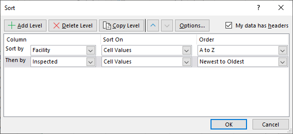
Figure 1. The Sort dialog box.

5. Click OK to actually sort the data.
6. With the Data tab of the ribbon still visible, click the Remove Duplicates tool in the Data Tools group. Excel displays the Remove Duplicates dialog box.
7. Make sure that the only field selected in the dialog box is the one that contains the facility. (See Figure 2.)



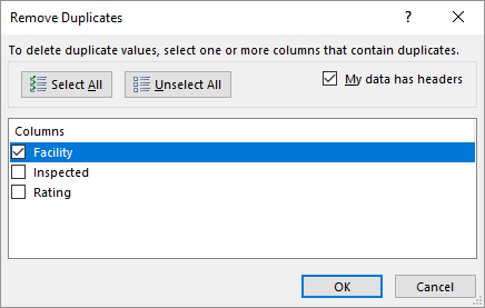
Figure 2. The Remove Duplicates dialog box.

8. Click OK. Excel removes the duplicates and leaves only those records that contain the latest (most recent) inspection date.

Understand that if you follow these steps it is destructive to your data—when completed, the older data is completely removed from your worksheet. Thus, if you want to maintain the older information for historical purposes, you may want to perform the steps on a duplicate of your data.

Of course, you could also use a different approach that maintains the original data and simply extracts the information that represents the latest inspection dates. Assume, for the purposes of this example, that your data is in columns A:C, with A containing the facility, B containing the inspection date, and C containing the rating achieved on that date. Further, the first row of your data contains headings (Facility, Inspected, and Rating). Somewhere to the right of your data—separated by at least one empty column—place another set of identical headings. (For this example I'll assume that these appear columns E:G.)

In the first column place a unique list of your facilities. In cell F2 place the following formula:

=MAX(($A$2:$A$123=E2)*$B$2:$B$123)

You can replace the two lower range references ($A$123 and $B$123) with whatever lower range is appropriate for your data. Also, you need to enter this as an array formula, meaning you press Ctrl+Shift+Enter to add it to cell F2.

The result in cell F2 will be a number, which is actually a date. (Excel maintains dates internally as numbers.) To get F2 to look like a date, simply apply a date format to the cell.

In cell G2 place the following formula:

=SUMIFS($C$2:$C$123,$A$2:$A$123,E2,$B$2:$B$123,F2)

Again, the lower range references can be replaced with whatever reference is appropriate for your data. This is not an array formula, so you can simply press Enter to put it in cell G2.

Now copy cells F2:G2 down as many rows as appropriate for your facilities. What you end up with is a dynamic list of the most recent inspection results for each facility. (See Figure 3.)

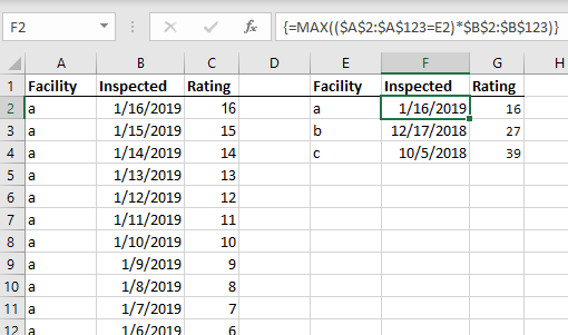
Figure 3. A dynamic list of the latest inspection results.

As you add more data to your inspection list, your "result table" is updated to always show the latest inspection results.

ExcelTips is your source for cost-effective Microsoft Excel training. This tip (13125) applies to Microsoft Excel 2007, 2010, 2013, 2016, 2019, 2021, 2024, and Excel in Microsoft 365.