Dutch has a worksheet he uses to track all of the cruises he has taken. Each row is one cruise. The left-hand columns contain ship name, departure date, booking number, etc. The ten right-most columns are labeled "Port 1" through "Port 10" to record the ports visited, in order. Nassau, for instance, might be the first stop on one cruise and the third stop on another. Dutch can't figure out a simple, straightforward way to use a PivotTable (as he does, e.g., to see how many times he's cruised on a particular ship, etc.) to see how many times he's visited each port. He wonders if a PivotTable can be used to count the number of times each unique value appears in a range of cells as opposed to a single row or column.
Dutch can solve this problem without even resorting to a PivotTable. This can be done by selecting the cells containing the ports and giving that range a name, such as "Ports." (How you set up a named range has been covered in other ExcelTips.)
At this point there are two ways you can go, depending on your version of Excel. If you are using Excel 2024 or Microsoft 365, you can use the following to provide a list of all the port names:
=SORT(UNIQUE(TOCOL(Ports,1)))
If you are using an older version of Excel, then the list will need to be manually created. The list could be placed on the same worksheet that Dutch is using, or it could be on a different worksheet in the same workbook.
Let's say, for instance, that the port names are in column A, starting below the detailed data in row 22. To the right of the port names, in column B, you could add a simple COUNTIFS formula that references the named range you created:
=COUNTIFS(Ports, A22)
Copy this down as many cells as necessary, and you will have a count of how many times each port was visited. (See Figure 1.)
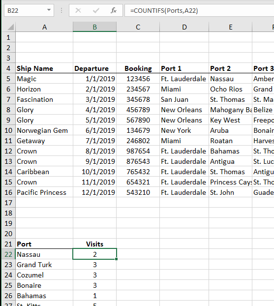
Figure 1. Getting a Count of Ports
The downside to this approach, of course, is that you'll need to make sure that the Ports named range refers to the proper range whenever you add new cruises. You'll also need to manually add any ports desired to the port list if you are using Excel 2019 or older.
Of course, you can bypass putting a formula in column B completely, provided you are using Excel 2024 or Microsoft 365. It just takes a slightly different formula in cell A22:
=LET(x,TOCOL(Ports,1),y,SORT(UNIQUE(x)),HSTACK(y,COUNTIFS(Ports,y)))
This single formula provides the port list and the count for each port.
If you absolutely want to use a PivotTable, then you will need to restructure your data. PivotTables are used to analyze the contents of rows and columns, as implied in Dutch's original question about whether a range could be analyzed. So, instead of having 10 columns to track each port of call, you could have multiple rows that define each cruise, with each row being a port of call. (See Figure 2.)
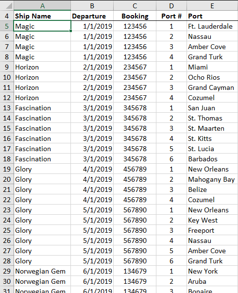
Figure 2. Reorganizing Your Data
With the data in a format such as this, you can easily create a PivotTable based on the contents of the Port column that would show the count for each port visited. Restructuring in this way—with each row being a port visited—makes the data much more conducive to analyzing with a PivotTable.
ExcelTips is your source for cost-effective Microsoft Excel training. This tip (13625) applies to Microsoft Excel 2007, 2010, 2013, 2016, 2019, 2021, 2024, and Excel in Microsoft 365.

Professional Development Guidance! Four world-class developers offer start-to-finish guidance for building powerful, robust, and secure applications with Excel. The authors show how to consistently make the right design decisions and make the most of Excel's powerful features. Check out Professional Excel Development today!
You can format PivotTables using either manual formatting or automatic formatting. You need to be careful, however, as ...
Discover MorePivotTables are used to analyze huge amounts of data. The number of rows used in a PivotTable depends on the type of ...
Discover MoreExcel allows you to link to values in other workbooks, even if those values are in PivotTables. However, Excel may ...
Discover MoreFREE SERVICE: Get tips like this every week in ExcelTips, a free productivity newsletter. Enter your address and click "Subscribe."
2026-05-13 15:19:13
J. Woolley
The Tip uses this formula in cell B22
=COUNTIFS(Ports, A22)
but this formula might be more appropriate
=COUNTIF(Ports, A22)
And if the list of unique ports starting in A22 is the result of this formula
=SORT(UNIQUE(TOCOL(Ports, 1)))
then this formula can be used in cell B22
=COUNTIF(Ports, A22#)
Finally, the Tip suggests this formula in cell A22 returning a two column array
=LET(x,TOCOL(Ports,1),y,SORT(UNIQUE(x)),HSTACK(y,COUNTIFS(Ports,y)))
but here's an alternative with the same result (sorted by Port name)
=LET(a, SORT(UNIQUE(TOCOL(Ports, 1))), HSTACK(a, COUNTIF(Ports, a)))
Or you could sort by number of visits (descending)
=LET(a, UNIQUE(TOCOL(Ports, 1)), SORT(HSTACK(a, COUNTIF(Ports, a)), 2, -1))
Got a version of Excel that uses the ribbon interface (Excel 2007 or later)? This site is for you! If you use an earlier version of Excel, visit our ExcelTips site focusing on the menu interface.
FREE SERVICE: Get tips like this every week in ExcelTips, a free productivity newsletter. Enter your address and click "Subscribe."
Copyright © 2026 Sharon Parq Associates, Inc.
Comments