Garret received a bunch of data from his corporate computer system, and he needs to split it out into columns. A single cell might look like this:
"Working, August 2023", "Research, March 2024, Pending", "Offer, July 2023"
All text between each pair of quote marks should be in its own column, so he needs to split this to three columns and get rid of the quote marks. Garret thought he could use Text to Columns to split the original cell, but he cannot do it based on commas as a delimiter (since there are six commas in the source cell). Garret wonders about the easiest way to split out the nearly 5,000 cells he needs to work with.
There are several ways that this task can be approached. Perhaps the easiest way is to follow these general steps:
These three general steps work because the only place where a comma appears right after a quote mark is between what will eventually be columns. If you replace that comma (the one right after the quote mark) with a delimiter other than a comma, then you can use Text to Columns.
If you don't want to do a Find and Replace operation, you can still use Text to Columns. Follow these steps:
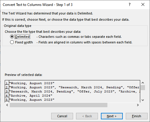
Figure 1. Convert Text to Columns Wizard, step 1.
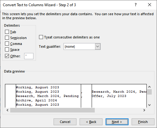
Figure 2. Convert Text to Columns Wizard, step 2.
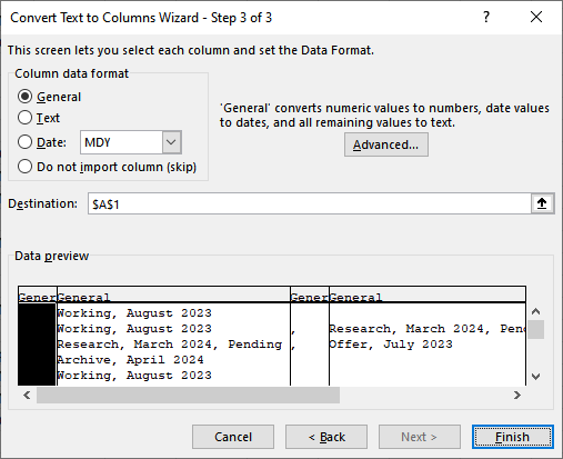
Figure 3. Convert Text to Columns Wizard, step 3.
You can also, if you are using Excel 2010 or a later version, use Power Query to import your data. Rather than walk through the steps necessary to set up the query, I'll choose to include here just the MCode for the query. (You can load the MCode using the advanced Power Query Editor.)
let
    Source = Excel.CurrentWorkbook(){[Name="Table1"]}[Content],
    #"Changed Type" = Table.TransformColumnTypes(Source,{{"Column1", type text}}),
    #"Split Column by Delimiter" = Table.SplitColumn(#"Changed Type", "Column1", Splitter.SplitTextByDelimiter(""", ", QuoteStyle.None), {"Column1.1", "Column1.2", "Column1.3", "Column1.4"}),
    #"Changed Type1" = Table.TransformColumnTypes(#"Split Column by Delimiter",{{"Column1.1", type text}, {"Column1.2", type text}, {"Column1.3", type text}, {"Column1.4", type text}}),
    #"Replaced Value" = Table.ReplaceValue(#"Changed Type1","""","",Replacer.ReplaceText,{"Column1.1", "Column1.2", "Column1.3", "Column1.4"})
in
    #"Replaced Value"
The MCode will handle up to four possible columns being extracted from the original data. It does require that you format your original data as a table and that it have the name Table1.
If you would like a macro to do the data conversion for you, then the following will do the trick for any number of final columns:
Sub ParseIt()
    Range(Selection, Selection.End(xlDown)).Select

    With Selection
        .Replace What:=""", """, Replacement:="~", LookAt:=xlPart
        .Replace What:="""", Replacement:="", LookAt:=xlPart
        .TextToColumns Destination:=ActiveCell, DataType:=xlDelimited, _
          Other:=True, OtherChar:="~", _
          FieldInfo:=Array(Array(1, 1), Array(2, 1), Array(3, 1))
    End With
    Range(Selection, Selection.End(xlToRight)).Select
    Selection.EntireColumn.AutoFit
    ActiveCell.Select
End Sub
In order to use the macro, all you need to do is to load your data and then select the first cell in the data.
Finally, if you are using Excel in Microsoft 365, Excel 2019, or Excel 2021, then you can use a formula to pull apart your original data. Assuming your data starts in cell A1, place this formula in a row-1 cell to the right of your data:
=SUBSTITUTE(TEXTSPLIT(A1,""", """),"""","")
Copy the formula down as far as necessary and you'll have your split-out data.
Note:
ExcelTips is your source for cost-effective Microsoft Excel training. This tip (13906) applies to Microsoft Excel 2007, 2010, 2013, 2016, 2019, 2021, and Excel in Microsoft 365.

Dive Deep into Macros! Make Excel do things you thought were impossible, discover techniques you won't find anywhere else, and create powerful automated reports. Bill Jelen and Tracy Syrstad help you instantly visualize information to make it actionable. You�ll find step-by-step instructions, real-world case studies, and 50 workbooks packed with examples and solutions. Check out Microsoft Excel 2019 VBA and Macros today!
The easy way to get rid of spaces at the beginning or end of a cell's contents is to use the TRIM function. ...
Discover MoreExcel allows you to easily paste information into a worksheet, including through simply dragging and dropping the ...
Discover MoreEdit a group of workbooks at the same time and you probably will find yourself trying to copy information from one of ...
Discover MoreFREE SERVICE: Get tips like this every week in ExcelTips, a free productivity newsletter. Enter your address and click "Subscribe."
2023-08-17 12:43:58
Willy Vanhaelen
@Tomek
It is because in your previous comment you pointed to the right direction that I started to try out several combinations that lead to this easy and simple procedure. I also got a better insight in the text to column wizard and the CSV file format I hardly used in the past.
Obviously, an update of this tip is unavoidable.
2023-08-15 11:41:28
Tomek
@Willy Vanhaelen and @Allen:
Re: Comment of 2023-08-14 12:06:23
BINGO!
No need to do any replacement!
And good learning about how the text inside the quotes is treated when splitting Text-to-Columns.
@Allen:
It may be worthwhile to update your tip with this simplest solution.
2023-08-14 12:06:23
Willy Vanhaelen
@Tomek
While trying out what you explained in your second paragraph, I discovered an even much easier procedure:
I selected the comma AND space as delimiters AND checked the quote mark as text qualifier and then clicked Finish and the job was done !!!
It seems that Excel sees the comma/space combination as the delimiter but only if they are outside the quote marks. So, there is even no need for the tilde ~.
There is even no need for a macro either.
2023-08-13 20:43:57
Hopefully a better quality screenshot (see Figure 1 below)
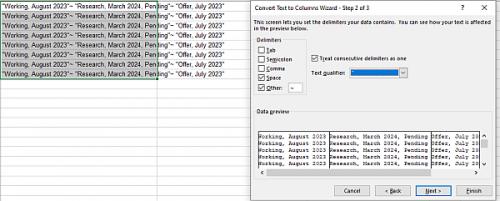
Figure 1.
2023-08-13 20:35:58
@Willy Vanhaelen comment of 2023-08-05 12:03:17
As I mentioned in my comment, leaving the space in will interfere with the Text-to-Columns operation. If you remove the spaces after the commas, and do Text-toColumn with ~ as delimiter ***AND*** quotation mark (") as Text qualifier - the quotation marks will be removed; no need to remove them by another Find and Replace. If you leave the spaces after the commas, only the first pair of the quotation marks will be removed, the rest, as the quotation mark in each of them will be preceded by a space, will get Excel "confused" and the remaining quotation marks will stay.
I got some success without removing the spaces, but with setting the delimiter to "~" and <space> at the same time, with "Treat consecutive delimiters as one" checked ***AND*** (") as text qualifier. Somewhat surprisingly, this did not treat the spaces inside the quotation marks as delimiters! I guess the text within quotes was identified as one indivisible piece. See a sample screenshot - (see Figure 1 below)
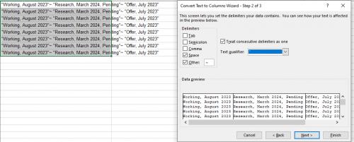
Figure 1.
2023-08-13 12:22:14
Willy Vanhaelen
To use the macro, select your one column range, and run it.
2023-08-13 12:13:44
Willy Vanhaelen
This tip’s macro does the job very well. It occurred to me though that the two functions (Replace and TextToColumns) used in the For Each loop are in fact Excel functions. So, I thought that, as an experiment, it would be interesting to make a macro based on pure VBA functions. I managed to do it by using 2 InStr(Rev) and 3 Mid functions. This is the result:
Sub txt2col()
Dim cell As Range, X As Integer, Y As Integer, Z As Integer
X = Selection.Column
For Each cell In Selection
Y = InStrRev(cell, """, """)
Cells(cell.Row, X + 2) = Mid(cell, Y + 4, Len(cell) - Y - 4)
Z = InStr(cell, """, """)
Cells(cell.Row, X + 1) = Mid(cell, Z + 4, Y - Z - 4)
cell = Mid(cell, 2, Z - 2)
Next cell
Y = Selection.Row
Range(Cells(Y, X), Cells(Y, X + 2)).EntireColumn.AutoFit
End Sub
2023-08-06 10:37:28
J. Woolley
The Tip's final dynamic array formula
=SUBSTITUTE(TEXTSPLIT(A1,""", """),"""","")
refers to "Excel in Microsoft 365, Excel 2019, or Excel 2021," but TEXTSPLIT is only in 365 and 2019 does not support dynamic arrays.
My Excel Toolbox includes the following function:
=SplitText(Text,[Delimiter],[CaseSensitive],[Limit],[Remainder])
This returns an array of substrings after dividing Text at each occurrence of Delimiter; the default Delimiter is a space character, but any string is permitted. If CaseSensitive is FALSE (default), alphabetic case of Delimiter is ignored. If Limit = -1 or TRUE (default), all substrings are returned; otherwise, the result has Limit substrings (which must be > 0). If Remainder is FALSE (default) and Limit > 0, any remainder is ignored; otherwise, the last substring will include the remainder. Here is an abbreviated version:
Public Function SplitText(Text As String, Optional Delimiter As String = " ", Optional CaseSensitive As Boolean = False, Optional Limit As Integer = -1, Optional Remainder As Boolean = False) As String()
Dim n As Integer, A() As String
n = IIf(Remainder Or (Limit < 1), Limit, (Limit + 1))
A = Split(Text, Delimiter, n, _
IIf(CaseSensitive, vbBinaryCompare, vbTextCompare))
n = UBound(A)
If (Not Remainder) And (Limit > 0) And (n >= Limit) Then _
ReDim Preserve A(n - 1)
SplitText = A
End Function
Assuming the Tip's data starts in cell A1 and its quoted substrings are separated by comma plus space (2 characters), this Excel 2021+ dynamic array formula will spill the split results into empty cells on the right:
=SUBSTITUTE(SplitText(A1,""", """),"""","")
With CHAR(34) as quotation mark, CHAR(44) as comma, and CHAR(32) as space, here is the equivalent formula, which might be easier to understand:
=SUBSTITUTE(SplitText(A1,CHAR(34)&CHAR(44)&CHAR(32)&CHAR(34)),CHAR(34),"")
The Tip's data contains only 3 quoted substrings; therefore, the following CSE array formula can be used in older versions of Excel by selecting 3 empty columns and pressing Ctrl+Shift+Enter:
=SUBSTITUTE(SplitText(A1,""", """,,3,TRUE),"""","")
And here is the equivalent formula:
=SUBSTITUTE(SplitText(A1,CHAR(34)&CHAR(44)&CHAR(32)&CHAR(34),,3,TRUE),CHAR(34),"")
As stated in the Tip, "Copy the formula down as far as necessary and you'll have your split-out data." For the CSE array formula, you must select all 3 columns before copying.
See https://sites.google.com/view/MyExcelToolbox/
2023-08-05 12:03:17
Willy Vanhaelen
@Tomek
You are right, the first method doesn’t remove the space following the comma but it also doesn’t get rid of the quote marks. Here is the correction:
2. Do a Find and Replace operation, replacing a quote mark followed by a comma AND A SPACE (", “) by simply a tilde (~) ...
2 bis. CONTINUE IN FIND AND REPLACE TO REMOVE ALL THE QUOTE MARKS: in “Find What:” replace (", ) with one quote mark and delete the ~(tilde) in “Replace with:”.
2023-08-05 07:20:03
Tomek
In the first method, it is beneficial to replace also the space following the comma, i.e., use (", ) as Find what, and replace it with ("~). This will remove the space after the comma, that is present in Garret's data. If you leave the space in, it may interfere with the split.
Also, when selecting the delimiter (~), make sure that (") is selected as Text qualifier; this will result with quotation marks to be removed from the split columns.
Got a version of Excel that uses the ribbon interface (Excel 2007 or later)? This site is for you! If you use an earlier version of Excel, visit our ExcelTips site focusing on the menu interface.
FREE SERVICE: Get tips like this every week in ExcelTips, a free productivity newsletter. Enter your address and click "Subscribe."
Copyright © 2026 Sharon Parq Associates, Inc.
Comments