Rounding to a Half Hour and Formatting the Display

Lorene has a column that contains various times of day. She needs to round the times to the nearest half hour and display them as, for example, 10 am and 10:30 am. (Lowercase, minutes shown for only the half hour, and lowercase am/pm indicator.) She wonders if this is something she can do with a custom format, or if she needs to use a formula.

The short answer is that you cannot get the desired result with just a custom format. Instead, you'll need to use three features of Excel: a formula, a custom format, and a conditional format, all working in conjunction with each other. How you can round times has been covered in a different ExcelTip, here:

https://tips.net/T11401

To boil it down succinctly, in Lorene's case you could round the time to the nearest half hour in the following manner:

=MROUND(A1,"0:30")

This assumes, of course, that the original time is in cell A1. You can then apply the following custom format to the result of the formula:

h:mm a/p\m

This will display the results of the formula as hours and minutes with an am/pm indicator. This, however, still isn't quite what Lorene is looking for, which is no minutes indicated if the minutes are ":00". The final step can be accomplished by adding a conditional format to the cell. Assuming that your formula is in cell B1, follow these steps:

1. Select cell B1.
2. Make sure the Home tab of the ribbon is displayed.
3. Click the Conditional Formatting tool. Excel displays a series of choices.
4. Click New Rule. Excel displays the New Formatting Rule dialog box.
5. In the Select a Rule Type area at the top of the dialog box, choose Use a Formula to Determine Which Cells to Format. (See Figure 1.)



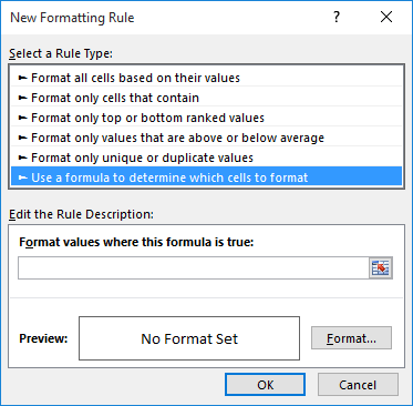
Figure 1. The New Formatting Rule dialog box.

6. In the formula space, enter the following formula:

     =MINUTE(B1)=0

7. Click on the Format button. Excel displays the Format Cells dialog box.
8. Make sure the Number tab is selected.
9. Click Custom at the bottom-left side of the dialog box. (You are setting a custom format to be used if the formula in step 6 is True.)
10. In the Type box, enter the following format:

     h a/p\m

11. Click OK to close the Format Cells dialog box.
12. Click on OK to close the New Formatting Rule dialog box.

That's it; the cell will now display the formatted time value as Lorene desired.

ExcelTips is your source for cost-effective Microsoft Excel training. This tip (13913) applies to Microsoft Excel 2007, 2010, 2013, 2016, 2019, Excel in Microsoft 365, and 2021.