Unwanted Hyperlinks

One of the things that Excel does automatically is to recognize URLs and e-mail addresses as something special. When you input one of these, Excel formats it as an active hyperlink. This behavior can be rather bothersome, particularly if you need to enter quite a few e-mail addresses or URLs in Excel.

There are several ways you can get around this behavior. The first (and perhaps easiest method) is to simply change the way in which you input URLs and e-mail addresses. When you enter one, start it with an apostrophe. Thus, instead of entering jdoe@xyz.com, I would enter 'jdoe@xyz.com. The only difference is the leading apostrophe. Excel does not display the apostrophe in the worksheet, only in the formula bar. In addition, the address is treated like any other text in the worksheet.

The second method is to go ahead and input your address (e-mail or URL) as you normally would. When you press Enter or Tab to move to the next cell, Excel formats the address as a hyperlink. If you immediately press Ctrl+Z, the hyperlink is removed, but the address remains.

Another method is to simply remove the hyperlink after it is created by Excel. To do this, just right-click on the hyperlink and then choose Remove Hyperlink from the resulting Context menu.

You can also turn off automatic hyperlink creation. Follow these steps:

1. Display the Excel Options dialog box. (In Excel 2007 click the Office button and then click Excel Options. In Excel 2010 or a later version, display the File tab of the ribbon and then click Options.)
2. Click Proofing at the left side of the dialog box.
3. Click AutoCorrect Options. Excel displays the AutoCorrect dialog box.
4. Make sure the AutoFormat As You Type tab is selected. (See Figure 1.)



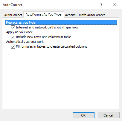
Figure 1. The AutoFormat As You Type tab of the AutoCorrect dialog box.

5. Clear the Internet and Network Paths with Hyperlinks check box.
6. Click OK to close the AutoCorrect dialog box.
7. Click OK to close the Excel Options dialog box.

ExcelTips is your source for cost-effective Microsoft Excel training. This tip (8666) applies to Microsoft Excel 2007, 2010, 2013, 2016, 2019, and 2021. You can find a version of this tip for the older menu interface of Excel here: Unwanted Hyperlinks.