Please Note: This article is written for users of the following Microsoft Excel versions: 2007, 2010, 2013, 2016, 2019, and 2021. If you are using an earlier version (Excel 2003 or earlier), this tip may not work for you. For a version of this tip written specifically for earlier versions of Excel, click here: Extracting Targeted Records from a List.
Written by Allen Wyatt (last updated August 7, 2025)
This tip applies to Excel 2007, 2010, 2013, 2016, 2019, and 2021
In a business environment, it is not unusual to use Excel to help manage the data you need to work with every day. For instance, you may use Excel to "crunch" invoice data, shipping records, or any number of different types of data. When working with that data, you may need to extract different records based upon particular criteria.
This is where the filtering capabilities of Excel come in handy. Consider the scenario where you have several thousand orders, covering customers across the country. You may want to extract the orders that belong to customers in targeted states so that you can process them first. You can do this using the advanced filtering capabilities of Excel. (For these steps, assume that the data you want to filter is in columns A through K.)
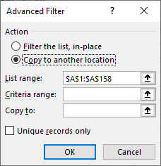
Figure 1. The Advanced Filter dialog box.
That's it—Excel copies those records that have one of your target states to whatever location you specified in step 9, and the original data is left unchanged.
ExcelTips is your source for cost-effective Microsoft Excel training. This tip (6116) applies to Microsoft Excel 2007, 2010, 2013, 2016, 2019, and 2021. You can find a version of this tip for the older menu interface of Excel here: Extracting Targeted Records from a List.

Solve Real Business Problems Master business modeling and analysis techniques with Excel and transform data into bottom-line results. This hands-on, scenario-focused guide shows you how to use the latest Excel tools to integrate data from multiple tables. Check out Microsoft Excel Data Analysis and Business Modeling today!
Given a long list of names, part numbers, or what-have-you, you may need to determine the unique values within the list. ...
Discover MoreMany people know how to use AutoFilter, but there are times when you need some more filtering muscle. Here's how you can ...
Discover MoreFREE SERVICE: Get tips like this every week in ExcelTips, a free productivity newsletter. Enter your address and click "Subscribe."
2025-08-07 14:52:17
Cheryl olsen
Really useful! Thanks. I have taken your courses and find the very useful, especially pivot tables
Got a version of Excel that uses the ribbon interface (Excel 2007 or later)? This site is for you! If you use an earlier version of Excel, visit our ExcelTips site focusing on the menu interface.
FREE SERVICE: Get tips like this every week in ExcelTips, a free productivity newsletter. Enter your address and click "Subscribe."
Copyright © 2026 Sharon Parq Associates, Inc.
 Please Note:
This article is written for users of the following Microsoft Excel versions: 2007, 2010, 2013, 2016, 2019, and 2021. If you are using an earlier version (Excel 2003 or earlier), this tip may not work for you. For a version of this tip written specifically for earlier versions of Excel, click here:
Please Note:
This article is written for users of the following Microsoft Excel versions: 2007, 2010, 2013, 2016, 2019, and 2021. If you are using an earlier version (Excel 2003 or earlier), this tip may not work for you. For a version of this tip written specifically for earlier versions of Excel, click here:
Comments