Highlighting Cells with Text Over a Certain Length

Bonnie has a worksheet that contains a large number of text values. She wonders if it is possible to use a conditional format to highlight cells that contain text that is longer than 25 characters. Due to restrictions at her company, she needs to do this without using a macro.

This is quite easy to do without a macro, but you do need to set up a conditional formatting rule that relies on a formula. Follow these steps:

1. Select the cells that contain the text values.
2. Display the Home tab of the ribbon.
3. Click on the Conditional Formatting tool. Excel displays a group of options.
4. Choose the New Rule option. Excel displays the New Formatting Rule dialog box.
5. In the Select a Rule Type area at the top of the dialog box, choose Use a Formula to Determine Which Cells to Format. Excel changes the appearance of the New Formatting Rule dialog box. (See Figure 1.)



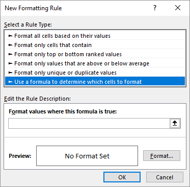
Figure 1. The New Formatting Rule dialog box.

6. In the formula space, enter the following formula: =LEN(A1)>25
7. Click on Format and use the formatting controls to indicate how you want cells formatted.
8. Click on OK. Excel saves and immediately applies the conditional formatting rule.

The formula you use in step 6 should reference the active cell in the range you selected in step 1. In this example, it assumes that the active cell is A1, but you should replace it with the cell that is appropriate for the cells you selected. In addition, you can modify the number of characters from 25 to whatever fits your needs.

If it is possible that some of the cells in the range could contain numeric values, then you may want the change the step 6 formula slightly:

=AND(ISTEXT(A1),LEN(A1)>25)

The formula checks that the cell contains text and its length. In this case, there are two references to cell A1 that should be modified to reflect the active cell in the cell range you selected.

ExcelTips is your source for cost-effective Microsoft Excel training. This tip (13460) applies to Microsoft Excel 2007, 2010, 2013, 2016, 2019, 2021, 2024, and Excel in Microsoft 365.