Shading Based on Odds and Evens

If you have a series of values in a range of cells, you might want to use different formatting to differentiate the odd numbers from the even numbers. The way you do this is through the use of the Conditional Formatting feature in Excel. Follow these steps:

1. Select the cells that contain the odd and even values.
2. With the Home tab of the ribbon displayed, click the Conditional Formatting option in the Styles group. Excel displays a palette of options related to conditional formatting.
3. Click Manage Rules. Excel displays the Conditional Formatting Rules Manager dialog box.
4. Click New Rule. Excel displays the New Formatting Rule dialog box.
5. In the Select a Rule Type area at the top of the dialog box, choose Use a Formula to Determine Which Cells to Format. (In Excel 2013 and later versions, click on New Rule and then select Use a Formula to Determine Which Cells to Format.) (See Figure 1.)



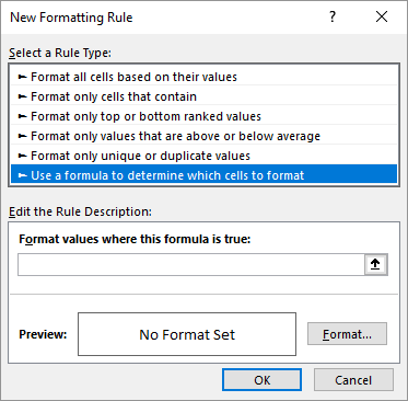
Figure 1. The New Formatting Rule dialog box.

6. In the Format Values Where This Formula Is True box, enter the following: =MOD(A1,2)=1. This formula will return True if the cell contains an odd value. (If the range of cells you selected in step 1 did not begin with cell A1, then change the formula to reflect the cell at the upper-left corner of your selected range.)
7. Click Format to display the Format Cells dialog box.
8. Using the controls in the dialog box, specify a format that you want used for those cells that contain an odd value.
9. Click OK to dismiss the Format Cells dialog box. The formatting you specified in step 7 should now appear in the preview area for the rule.
10. Click OK. The New Formatting Rule dialog box disappears and Excel again displays the Conditional Formatting Rules Manager dialog box. The rule you just defined is listed in the dialog box.
11. Repeat steps 4 through 10 for the second condition, but use the formula =MOD(A1,2)=0. This formula returns True if the cell contains an even value.
12. Click the up and down arrows to move the rules you created to the order in which they should be evaluated.
13. Click OK. Excel applies the conditional formatting to the cells you selected in step 1.

With this conditional formatting applied, if the cell is odd it will be one color and if even it will be another. If the cell contains text, the cell will be uncolored, meaning it will have the color of the cell before you added the conditional formatting. The conditional formatting overrides any formatting you put on the cell, so even if you try to change the cell color via the tools on the ribbons, the conditional formatting takes precedence.

The MOD function isn't the only thing you can use in your formula. If you want to determine whether the cell contains an odd value (step 6), you could use the following:

=ISODD(A1)

Similarly, if you want to determine if the cell contains an even value (step 11), you could use the following:

=ISEVEN(A1)

ExcelTips is your source for cost-effective Microsoft Excel training. This tip (6260) applies to Microsoft Excel 2007, 2010, 2013, 2016, 2019, Excel in Microsoft 365, and 2021. You can find a version of this tip for the older menu interface of Excel here: Shading Based on Odds and Evens.