Written by Allen Wyatt (last updated September 5, 2020)
This tip applies to Excel 2007, 2010, 2013, 2016, 2019, and 2021
Bill has a column of text in which he needs to replace all instances of letters with the number that represents the position of the letter in the alphabet. So, for instance, if a cell contains "T10A22", then Bill needs to replace the letters such as "2010122", where T is replaced with 20 and A is replaced with 1. He notes that there can be any number of letters in any given cell.
If you need to do this only once (in a single worksheet), it might be easy enough to select the column and just use Find and Replace. You can search for A and replace with 1, search for B and replace with 2, and so on. There would only be 26 iterations to perform, which might sound onerous but can be done in less time than it takes to create a macro to do the changes.
That being said, if you have to perform this task regularly, then a macro is your best solution. You can implement the Find and Replace approach using a macro in this manner:
Sub ReplaceLetters1()
    Selection.Replace What:="A", Replacement:="1", LookAt:=xlPart, _
      SearchOrder:=xlByRows, MatchCase:=False, SearchFormat:=False, _
      ReplaceFormat:=False, FormulaVersion:=xlReplaceFormula2
    Selection.Replace What:="B", Replacement:="2"
    Selection.Replace What:="C", Replacement:="3"
    Selection.Replace What:="D", Replacement:="4"
    Selection.Replace What:="E", Replacement:="5"
    Selection.Replace What:="F", Replacement:="6"
    Selection.Replace What:="G", Replacement:="7"
    Selection.Replace What:="H", Replacement:="8"
    Selection.Replace What:="I", Replacement:="9"
    Selection.Replace What:="J", Replacement:="10"
    Selection.Replace What:="K", Replacement:="11"
    Selection.Replace What:="L", Replacement:="12"
    Selection.Replace What:="M", Replacement:="13"
    Selection.Replace What:="N", Replacement:="14"
    Selection.Replace What:="O", Replacement:="15"
    Selection.Replace What:="P", Replacement:="16"
    Selection.Replace What:="Q", Replacement:="17"
    Selection.Replace What:="R", Replacement:="18"
    Selection.Replace What:="S", Replacement:="19"
    Selection.Replace What:="T", Replacement:="20"
    Selection.Replace What:="U", Replacement:="21"
    Selection.Replace What:="V", Replacement:="22"
    Selection.Replace What:="W", Replacement:="23"
    Selection.Replace What:="X", Replacement:="24"
    Selection.Replace What:="Y", Replacement:="25"
    Selection.Replace What:="Z", Replacement:="26"
End Sub
To use the macro, just select the cells you want to process and then run it. You could, as well, use a different approach that relies on a For...Next loop, in this manner:
Sub ReplaceLetters2()
    Dim J As Integer

    Selection.Replace What:="A", Replacement:="1", LookAt:=xlPart, _
        SearchOrder:=xlByRows, MatchCase:=False, SearchFormat:=False, _
        ReplaceFormat:=False, FormulaVersion:=xlReplaceFormula2
    For J = 66 To 90
        Selection.Replace What:=Chr(J), Replacement:=J - 64
    Next J
End Sub
While the first .Replace operation could be placed inside the For...Next loop, I chose to keep it separate so that (at least to me) the loop appeared simpler. This is a stylistic choice more than anything else.
If, for some reason, you don't want to use the .Replace method, you could use the old fashioned approach of looking at each character in whatever you are evaluating. This is the approach used in this user-defined function:
Function LetterToNum(c As Range) As String
    Dim sRaw As String
    Dim J As Integer

    sRaw = UCase(c)
    For J = 1 To 26
        sRaw = Replace(sRaw, Chr(J + 64), J)
    Next J
    LetterToNum = sRaw
End Function
To use this function, simply put the following in your worksheet, where A1 is the cell you want to convert:
=LetterToNum(A1)
If you prefer not to use macros, then you could use a rather long formula to do the conversion of a cell:
=TEXTJOIN("",FALSE, IF(ISNUMBER(VALUE(MID(A1,SEQUENCE(1,LEN(A1)),1))), MID(A1,SEQUENCE(1,LEN(A1)),1), COLUMN(INDIRECT(MID(A1,SEQUENCE(1,LEN(A1)),1) & ":" & MID(A1,SEQUENCE(1,LEN(A1)),1)))))
This formula assumes that the text you want to convert is in cell A1. It basically looks at each character in the text string and determines if it is a digit or not. If it is, then it uses the original character; if it is not, then it uses INDIRECT function to determine a column based on the letter and then uses COLUMN to return a numeric value for that column. This is all then recombined using the TEXTJOIN function.
Note:
ExcelTips is your source for cost-effective Microsoft Excel training. This tip (7820) applies to Microsoft Excel 2007, 2010, 2013, 2016, 2019, and 2021.

Excel Smarts for Beginners! Featuring the friendly and trusted For Dummies style, this popular guide shows beginners how to get up and running with Excel while also helping more experienced users get comfortable with the newest features. Check out Excel 2019 For Dummies today!
If you create a user form in VBA that includes checkboxes, you may want to make the checkboxes larger. You can't adjust ...
Discover MoreHaving macros in multiple open workbooks can sometimes produce unexpected or undesired results. If your macros are ...
Discover MoreISBNs are used to uniquely identify books. You may need to know if an ISBN is valid or not, which involves calculating ...
Discover MoreFREE SERVICE: Get tips like this every week in ExcelTips, a free productivity newsletter. Enter your address and click "Subscribe."
2021-06-23 11:00:14
J. Woolley
@Roy and Alan Elston
You might be interested in the freely available SpillArray(V_Array) function in My Excel Toolbox. This function is useful in older versions of Excel that do not support dynamic arrays. It will determine and populate the spill range for array expression V_Array, simulating a dynamic array.
The SpillArray function is in module M_RunMacro. The MyToolbox.xlam add-in file includes everything in My Excel Toolbox.
See https://sites.google.com/view/MyExcelToolbox/
2020-09-17 03:24:04
Alex B
@Bill
I really don't understand why you would want to this but here are some options, depending on what the variables are.
The assumption is that the first character is always alpha or you will need to use an if statement.
Cell A$ contains your A1234
Basic assumes capital letter (A-Z) in position 1 and length fixed at 5 =(CODE(LEFT(A4,1))-64)&RIGHT(A4,4)
Cater for variable length =(CODE(LEFT(A4,1))-64)&RIGHT(A4,LEN(A4)-1)
Basic plus cater for A-Z AND a-z =(CODE(LEFT(UPPER(A4),1))-64)&RIGHT(A4,4)
Cater for variable length =(CODE(LEFT(UPPER(A4),1))-64)&RIGHT(A4,LEN(A4)-1)
2020-09-16 23:43:03
Bill Toney
Is there a simpler formula and definitely don’t want to run a macro.
What would the formula be if the letter was always first in the sequence (A1234)? And, there was always only one letter.
2020-09-12 08:30:34
Peter Atherton
Alan
Thanks for the lucid post
Cheers
2020-09-11 05:05:23
Hi Peter,
As I understood it, the Spill stuff is not a function. It is a functionality which allows doing away with the need to do the CSE stuff. What happens in the newest Excel versions is that any array information there will automatically “spill” over or “spill” out into adjoining cells as appropriate.
I think the full working Spill functionality is only available in most recent Excel versions.
But annoyingly they introduced some of the required changes in Excel’s working earlier. This cause inconsistencies between Excel version like the ones we experienced a while back where some versions of Excel require that extra
If({1},__)
trick to coerce out array results in some “Evaluate(“ “) one liner “ type macros.
More recent versions , ( not necessarily the newest ) , don’t need that coercing anymore, even though those newer versions may not have the full Spill functionality
Just another example of Microsoft making a mess when changing things.
Alan Elston
2020-09-09 18:26:53
Peter Atherton
Alan & Roy
I have not heard of the SPILL function before but recently I came across this thread using Dynamic Arrays with a couple of examples that work with xl 2016. Well worth a look and it would be interesting to know if they work with 2013. I haven't been able to incorporate them yet myself. Here's the link
https://exceloffthegrid.com/dynamic-arrays-and-vba-user-defined-functions-udfs/
Regards
2020-09-09 02:56:56
@Roy --- --- Interesting comments. ------ I have less experience with these things --------- Just out of passing interest ------ I started a discussion Thread on the Spill stuff and associated new functions ------ https://excelfox.com/forum/showthread.php/2308-Dynamic-Arrays-Spilling-alternative-to-type-2-CSE-Entry ------ You are very welcome to add any comments there ------ ( I am not sure what I will ever do with that Thread. For now it is just a scratch pad for discussions on the Spill stuff and associated new functions, that’s all ) --- Maybe one day I will get around to do some typical examples comparing things with and without spill, discussing work around to problems, bugs etc. --- At the moment I don’t have anything above 2013, so I can’t look in any detail yet at the newer stuff--- ( I just added a link to your comments there, hope that’s OK )Alan Elston
2020-09-08 13:22:43
Roy
@Alan Elston, and anyone else interested:
Yep, SPILL functionality is definitely a work in progress and unfortunately, Excel's history is that once "published" there are no major revisements. An example might be VLOOKUP() which really sang when Excel allowed the use of a table ("t" not "T") header (and row header for that matter, in HLOOKUP(), along with general use of the headers), to be used for the output column parameter. The standard (nowadays) shot to the gut when decrying use of VLOOKUP() always mentions how an added column can cause horrors. But when they removed the header use functionality, making VLOOKUP() a work in progress candidate, they did no work. So I'm not so sure they're gonna fix several major problems with SPILL formulas. I've had to resort to using workarounds to get, say, only 20 items displayed instead of all of them, and to get the first x number of candidate records or the last x number of them, mainly so that the output fits in my available output space rather than giving an error when I didn't leave space for all 23,496 results. WIP, but clearly will never be fixed. Why? Well, again, history, and also, they have bigger issues to solve with them, their not working in Tables being one.
But mostly, any time I suggest something online, I try to remember to offer a {CSE} alternative since many do not have the most recent versions. I'm given 2019 by the boss, so after a year-two years of offering new things to the "special people" I get to have "the not-most-recent version of things" too. I try to remember about which functions might not be in the earlier versions and speak to that too. But... I don't always remember or have time. Fortunately, someone usually picks up the baton.
If you are using the older versions, anyone that is, a number of pretty useful "modern" functions are available using the Excel 4 macros commands Named Ranges. I've always been convinced that one reason we never got a FORMULATEXT() type function was because you could do it with an Excel 4 macro command so I think they figured "Why bother?" (For that matter, although I shouldn't think you would, you can enable Excel 4 macro capability and actually write the macros.) I have used six of them since the old days as one of the first things I read when I found out there were Excel tip sites online told me how to do so. But you might find a few that give you unexpected usability, things Excel no longer does except with them. Newer version users can benefit too, it's just over the 30 years, many have learned VBA and things like FORMULATEXT() now exist.
I never really liked the {CSE} world, and like the concept of SPILL, but it needs a ton of improvement. Not just the above, say, including being useful in Tables, but simple things like working in a formula, always, not maybe. One thing they have improved is more functions seem to be able to access their elements. So VLOOKUP() is now able to access their elements where it did NOT when first issued to the not-special-people. I think INDEX() always has, but I don't use it as much as VLOOKUP() so not sure. Oddly, XLOOKUP() will not work properly with SPILL functions. One must specify both arrays fully and traditionally if the SPILL array is multi-column. Even when you want to lookup in the first column and return from the first column (pointless, but demonstrates the point): it is aware enough that there are multiple columns, but won't let the lookup use any of them from the SPILL side. MATCH() can't use it either so INDEX/MATCH is busted without a fully specified range. Mind you, they'd better be dynamic too since the SPILL array can adjust dynamically. But VLOOKUP() works with multi-column SPILL arrays so I guess in the long run, VLOOKUP() emerges as champ here... Like I say, a long way to go. I just hope they plan to go that long way and not their historical "No way at all once it's published."
I do love how it helps use of arrays in formulas, even though work is needed there.
2020-09-06 05:24:07
@Roy
Just my 2 cents on the Spill / CSE thing..
A lot of the new functions and the Spill ( that is to say no longer needing to “CSE it “) seem to be the more intuitive way things might have been done initially.
Assuming the original programmes were not idiots, then I would assume that there were good reasons for doing things originally in the less intuitive way, and which by design or otherwise, led to things like the CSE thing and the way VLookUp was organised.
I personally think the newer functions and the Spill are not worth the compatibility problems and god knows what other Bugs lie ahead with them.
It seems just another example of Microsoft working backwards or running out of things for their people to do, and so they just change things, usually for the worse.
Just my opinion, that’s all.
I personally try to develop everything in Office 2003 – 2007 and then rarely go past 2013. I put a lot of effort into keeping stable versions of 2010 working on any computer I have any responsibility for maintaining.
Alan Elston
2020-09-06 04:55:33
Roy
For those without SEQUENCE(), use:
COLUMN( INDIRECT( "1:" & LEN(A1) ))
to generate the same idea. (To use real estate right to left. To use up-down real estate, use ROW(). In either case, if you have a version without SEQUENCE(), it also does not have SPILL functionality, so you must use {CSE} for the formula and take up actual cells, rather than everything occuring in a single cell.)
A sidenote on the {CSE} thing: I've found that formulas using SPILL which fail as you reach a building point because the function you just fed them into does not SPILL, do NOT necessarily push that failure forward: if you later feed them into a function which does use SPILL, they seem to miraculously no longer fail. It's conceivable, though I guess I doubt it and I have not experimented as I'm not sure one CAN accurately experiment with a SPILL-enabled version, that a formula which would give a single interim result and therefore feed out a single result usually, might, if fed into further functions and finally entered as {CSE} in the end even though in a single cell, might activate the use of full internal arrays in the interim and therefore produce a full string in this kind of situation rather than a single value (so "2010122" here instead of "T"). Possibly.
So that's SEQUENCE() and SPILL. One other thing was there... ah: TEXTJOIN(). Use CONCAT(), which is available in 2016 and it will be exactly the same result. After all, in this problem, no delimiter is desired and there will be no empty spots to deal with. The string of "text1,text2,text3..." is identical. And in testing, it gives the same result. For that matter, CONCATENATE() will work if you are joining the range of cells your {CSE} formula used to produce the changed values, though you need literal cells, not a range expression ( so "C1,D1,E1" not "C1:E1") but it can be easily built using the simple string creation methods I earlier claimed exist.
2020-09-05 19:29:20
Roy
For those without SEQUENCE(), use:
COLUMN( INDIRECT( "1:" & LEN(A1) ))
to generate the same idea. (To use real estate right to left. To use up-down real estate, use ROW(). In either case, if you have a version without SEQUENCE(), it also does not have SPILL functionality, so you must use {CSE} for the formula and take up actual cells, rather than everything occuring in a single cell.)
A sidenote on the {CSE} thing: I've found that formulas using SPILL which fail as you reach a building point because the function you just fed them into does not SPILL, do NOT necessarily push that failure forward: if you later feed them into a function which does use SPILL, they seem to miraculously no longer fail. It's conceivable, though I guess I doubt it and I have not experimented as I'm not sure one CAN accurately experiment with a SPILL-enabled version, that a formula which would give a single interim result and therefore feed out a single result usually, might, if fed into further functions and finally entered as {CSE} in the end even though in a single cell, might activate the use of full internal arrays in the interim and therefore produce a full string in this kind of situation rather than a single value (so "2010122" here instead of "T"). Possibly.
So that's SEQUENCE() and SPILL. One other thing was there... ah: TEXTJOIN(). Use CONCAT(), which is available in 2016 and it will be exactly the same result. After all, in this problem, no delimiter is desired and there will be no empty spots to deal with. The string of "text1,text2,text3..." is identical. And in testing, it gives the same result. For that matter, CONCATENATE() will work if you are joining the range of cells your {CSE} formula used to produce the changed values, though you need literal cells, not a range expression ( so "C1,D1,E1" not "C1:E1") but it can be easily built using the simple string creation methods I earlier claimed exist.
2020-09-05 19:01:32
Roy
Sorry... forgot to fit this in:
The reason the formula's as compact as it is is because you include the numerals in the list as well as the letters. So everything is being looked up, instead of just the letters, and therefore you don't have to distinguish which characters to look up and which to leave in place.
2020-09-05 18:58:29
Roy
If you are willing to set up the table, like Raymond Guzman's, the following will use VLOOKUP() fairly compactly to do the trick:
=TEXTJOIN("","false", VLOOKUP( MID($D1,SEQUENCE(1,LEN($D1)),1), LookupTable, 2,FALSE))
Since the list here is simple and not going to be added to or edited, it is an ideal candidate for using simple string creation techniques to make an array string of it that can be put into a Named Range so it doesn't stick out, or offend sensibilities, by existing in cells somewhere in the spreadsheet. The following is the string. Obnoixious-looking, yes, but it was simple, and straightforward, to build:
= {"0","0";"1","1";"2","2";"3","3";"4","4";"5","5";"6","6";"7","7";"8","8";"9","9";"A","1";"B","2";"C","3";"D","4";"E","5";"F","6";"G","7";"H","8";"I","9";"J","10";"K","11";"L","12";"M","13";"N","14";"O","15";"P","16";"Q","17";"R","18";"S","19";"T","20";"U","21";"V","22";"W","23";"X","24";"Y","25";"Z","26"}
Keep the lookup table concept and populate it differently and you can use the concept for replacing other things. Examples could include replacing anything in a string not a number or number related (for example, keeping common arithmetic operators and things like "." and ",") — I do that for an end use no one would share although they might value it for other their own end uses — or perhaps building a list of non-printing white space characters you have encountered and would like to clean from your data much more comprehansively than something like "CLEAN()" does or even replacing accented characters with unaccented letters. Each list can be added to and edited over time, to suit.
If you had a lot of need for such and did not want them to bother users, you could have a separate spreadsheet in which you build them (again, a simple, straightforward process) and place them in Named Ranges in the spreadsheet given to users. Keep the building work (you know, one list to a worksheet, type any notes you might need for something that altered the normal step list) and you can easily add, edit, or remove and re-create the string, then copy that into the user spreadsheet Named Range, and voilà, all set.
In the meantime, pretty simple formula, using a pretty simple list, and therefore very easy to maintain, and also to pass on when you get a promotion. (Remember that about spreadsheets: don't ever make yourself unpromotable because no one can understand your spreadsheets so you always have to stay put... no one needs THAT kind of job security!)
2020-09-05 13:09:57
Robert Lohman
Willie, your formula works great as usual. I know my computer is not the fastest in town but this guy takes approx 12/13 seconds to compute just one cell . Any thoughts on how to reduce the run time?
2020-09-05 09:18:44
Alex B
And just because I have been looking for an excuse to try out a byte array, this also works.
Function LetterToNum(c As Range) As String
Dim i As Long
Dim x() As Byte
Dim a() As String
Dim sRaw As String
x = StrConv(UCase(c.Value), vbFromUnicode) ' Convert to ascii array
a = Split(StrConv(c.Value, vbUnicode), Chr(0)) ' Single character array
For i = 0 To UBound(x)
If x(i) > 64 And x(i) < 91 Then
sRaw = sRaw & x(i) - 64
Else
sRaw = sRaw & a(i)
End If
Next
LetterToNum = sRaw
End Function
2020-09-05 07:25:34
Raymond Guzman
Thanks for the tips, Allen.
For those of who can't use the macro option, please note that the SEQUENCE function is not available to Excel 2016 users. I tried to replace it with CONCATENATE, but was not able to use the SEQUENCE function - which is not available to some Excel 2016 users.
Since you credited me as a contributor to this solution, I would like to offer my suggestion.
(see Figure 1 below)
For each of the characters, you will have to prepare a formula to change text to a number if necessary.
The following assumes the text you are converting in Cell A1 and the alpha-numeric lookup text and values are in Columns J & K.
The 1st character will be analyzed on Cell B1 using:
=IF(ISTEXT(IFERROR(VALUE(MID($A1,1,1)),MID($A1,1,1)))=TRUE,IFERROR(VLOOKUP(MID($A1,1,1),$J:$K,2,0),""),VALUE(MID($A1,1,1)))
The 2nd character will be analyzed on Cell B1 using:
=IF(ISTEXT(IFERROR(VALUE(MID($A1,2,1)),MID($A1,2,1)))=TRUE,IFERROR(VLOOKUP(MID($A1,2,1),$J:$K,2,0),""),VALUE(MID($A1,2,1)))
The pattern can be continued for the next characters needed to be analyzed. These can then be joined, in this case in Cell using:
=B1&C1&D1&E1&F1&G1&H1
Regards and Happy Labor Day weekend,
Raymond Guzman
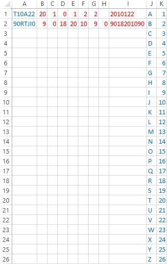
Figure 1. Location of analysis text, formulas, and lookups.
2020-09-05 06:32:50
Willy Vanhaelen
The ReplaceLetters1 macro can be much shorter using a loop:
Sub ReplaceLetters1b()
Dim X As Integer
Selection.Replace What:="A", Replacement:="1", LookAt:=xlPart, _
SearchOrder:=xlByRows, MatchCase:=False, SearchFormat:=False, _
ReplaceFormat:=False
For X = 2 To 26
Selection.Replace What:=Chr(X + 64), Replacement:=X
Next X
End Sub
Got a version of Excel that uses the ribbon interface (Excel 2007 or later)? This site is for you! If you use an earlier version of Excel, visit our ExcelTips site focusing on the menu interface.
FREE SERVICE: Get tips like this every week in ExcelTips, a free productivity newsletter. Enter your address and click "Subscribe."
Copyright © 2025 Sharon Parq Associates, Inc.
Comments