Getting a List of Matching Cells

When Michael does a "Find All" operation in Excel, the program helpfully shows a list of all the cells containing whatever he is searching for. Michael would like to copy that list of cell addresses into another worksheet, so he wonders if there is a way to copy the list to the Clipboard so he can paste it into a worksheet.

There are a few ways you can accomplish this task, and most of them involve the use of macros. Before getting to the macro-based approaches, however, let's take a look at way you could access the addresses using named ranges and the Name Manager:

1. Use FindAll as before, but don't close the Find and Replace dialog box.
2. In the list of addresses you are shown, scroll to the bottom, hold down the Shift key, and click on the last match. Excel selects all the matching cells.
3. Press Esc to close the Find and Replace dialog box. The matching cells are still all selected.
4. Type a name in the Name Box (just to the left of the Formula bar and just above cell A1). This creates a named range that consists of all the selected cells.
5. Display the Formulas tab of the ribbon.
6. Click the Name Manger tool. Excel displays the Name Manager's dialog box. (See Figure 1.)



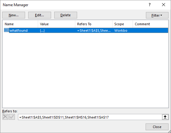
Figure 1. The Name Manager dialog box.

7. Click on the name you created in step 4.
8. The list of cells will be in the Refers To box, at the bottom of the dialog box.

At this point you can copy the information in the Refers To box and paste it into whatever you want (including another worksheet). You'll need to massage the data a bit after you paste it, as the list is just that—a serial list of cell addresses.

Obviously, this affects your workbook, as it creates a named range. If you do it multiple times, you'll have multiple named ranges created. This can, of course, quickly get unwieldy if you need to perform the task quite often. This is where the macro solutions come into play. The following is an example of a macro that will search for a specific value and then place the address of every cell containing that value into another worksheet.

Sub CellAdressList()
    Dim c1 As String
    Dim nxt As String

    Sheets("Sheet1").Select
    Range("A1").Select
    Cells.Find(What:="qrs", After:=ActiveCell, _
      LookIn:=xlValues, LookAt:=xlWhole, _
      SearchOrder:=xlByRows, SearchDirection:=xlNext, _
      MatchCase:=False, SearchFormat:=False).Activate
    c1 = ActiveCell.Address
    Sheets("Sheet2").Select
    Range("A1").Select
    Range("A1").Value = c1
    Do Until nxt = c1
        Sheets("Sheet1").Select
        Cells.FindNext(After:=ActiveCell).Activate
        nxt = ActiveCell.Address
        Sheets("Sheet2").Select
        ActiveCell.Offset(1, 0).Select
        ActiveCell.Value = nxt
    Loop
    ActiveCell.Value = ""
End Sub

The macro makes a few assumptions. First, it assumes that you are searching for information on the worksheet named Sheet1. Second, it assumes you want the list of addresses placed in the worksheet named Sheet2. Finally, it assumes you are searching for the value "qrs" within Sheet1. All of these elements of the macro can be changed, if desired.

For something just a bit more flexible, consider the following macro. It assumes that you have already selected all the cells that contain the value you want. (In other words, you need to perform steps 1 through 3 of the steps near the beginning of this tip.) You can then run the macro.

Sub CopyFindAllSelection()
    Dim outcell As Range
    Dim c As Range

    Set outcell = Range("Sheet2!A1")
    For Each c In Selection
        outcell.Value = c.Address
        Set outcell = outcell.Offset(1, 0)
    Next
End Sub

The result is that the addresses of the selected cells are placed into the Sheet2 worksheet. This macro is a bit more flexible because it allows you to find anything in any worksheet. The only part "hard coded" is the worksheet (Sheet2) into which the addresses are placed.

ExcelTips is your source for cost-effective Microsoft Excel training. This tip (13581) applies to Microsoft Excel 2007, 2010, 2013, 2016, 2019, and Excel in Microsoft 365.