Conditional Formatting with Data Imported from Access

Cory is having a problem getting his conditional formatting to work as desired with information imported into Excel from Access. The data being imported in a particular column can either be text (such as "17 U") or numeric (such as 32). The conditional format checks to see if the value in the cell is greater than zero, in which case the value is underlined. This won't work properly with the imported data because not only does Excel treat the text (17 U) as text, but it also treats the numeric (32) as text. This makes sense, since Excel treats the entire column as text rather than changing data format for each cell in the column.

There are a couple of ways you can fix this problem. One is to change the formula you are using in your conditional format. Instead of checking to see if the value is greater than zero, use the following formula (set the conditional check to "Format Is"):

=VALUE(E3) > 0

This formula uses the VALUE function to check what is in cell E3. If the contents are a number—even if it is formatted as text by Excel—then the formula returns True and the condition is met for the formatting. If the contents of E3 really are text (as in "17 U"), then the formula returns a #VALUE error, which does not satisfy the condition and the formatting is not applied.

Another approach is to force Excel to evaluate the imported cells and convert them to numeric values, if appropriate. An easy way to do this is as follows:

1. After importing the data, select a blank cell from a column outside the range of those you just imported.
2. Press Ctrl+C. This copies the contents of the cell (nothing) to the Clipboard.
3. Select the cells that you want evaluated by Excel. For instance, select the column that contains the text values and the numeric values formatted as text.
4. Display the Home tab of the ribbon.
5. Click the down-arrow under the Paste tool, and then choose Paste Special. Excel displays the Paste Special dialog box. (See Figure 1.)



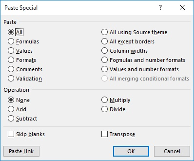
Figure 1. The Paste Special dialog box.

6. Click the Add radio button.
7. Click OK.

What you just did was to "add" the contents of the Clipboard to all the cells you selected in step 3. If the cells contained real text, then nothing happened to those cells; they remain the same and are still treated as text. If the cells contained a numeric value, then Excel treats it as a number and adds zero to it. This value, as a numeric, is deposited back in the cell, and treated as a real number. This means that the conditional formatting test that you previously set up should work just fine on those cells since they are no longer treated as text.

ExcelTips is your source for cost-effective Microsoft Excel training. This tip (5654) applies to Microsoft Excel 2007, 2010, 2013, 2016, 2019, and Excel in Microsoft 365. You can find a version of this tip for the older menu interface of Excel here: Conditional Formatting with Data Imported from Access.