Please Note: This article is written for users of the following Microsoft Excel versions: 2007, 2010, 2013, 2016, 2019, and 2021. If you are using an earlier version (Excel 2003 or earlier), this tip may not work for you. For a version of this tip written specifically for earlier versions of Excel, click here: Hiding Graphics.
Written by Allen Wyatt (last updated July 24, 2025)
This tip applies to Excel 2007, 2010, 2013, 2016, 2019, and 2021
If you are preparing worksheets that contain graphics, you may want to print the graphics on one version of the worksheet, but not print them on another. For example, you might be preparing a test for students, and the test requires them to draw a graph. You would want the printout of the student version of the test to leave space for drawing a graph, but the printout of the answer sheet should include the graphic showing how the students should answer.
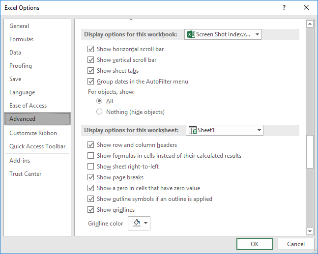
The easiest way to handle this in Excel is to just turn off display of the graphics when you need to print the student test. In order to do this, create a single file that contains the questions and the answers. Assuming the answers are graphic files, follow these steps:

Figure 1. The Advanced area of the Excel Options dialog box.
You can now print your document, as normal. (Excel prints it very quickly since it doesn't need to send the graphics to the printer.) When you later want to see the graphics, repeat the steps, but make sure you specify that Excel should display the objects, in step 5.
ExcelTips is your source for cost-effective Microsoft Excel training. This tip (6124) applies to Microsoft Excel 2007, 2010, 2013, 2016, 2019, and 2021. You can find a version of this tip for the older menu interface of Excel here: Hiding Graphics.

Program Successfully in Excel! This guide will provide you with all the information you need to automate any task in Excel and save time and effort. Learn how to extend Excel's functionality with VBA to create solutions not possible with the standard features. Includes latest information for Excel 2024 and Microsoft 365. Check out Mastering Excel VBA Programming today!
Want to change the way that a graphics object appears in your worksheet? You need to edit it, then, using the techniques ...
Discover MoreIf you use Excel's graphic capabilities to insert a line or an arrow into a worksheet, you can change how that arrow ...
Discover MoreIf you have a group of merged cells into which you want a user to enter information, you may want some sort of ...
Discover MoreFREE SERVICE: Get tips like this every week in ExcelTips, a free productivity newsletter. Enter your address and click "Subscribe."
There are currently no comments for this tip. (Be the first to leave your comment—just use the simple form above!)
Got a version of Excel that uses the ribbon interface (Excel 2007 or later)? This site is for you! If you use an earlier version of Excel, visit our ExcelTips site focusing on the menu interface.
FREE SERVICE: Get tips like this every week in ExcelTips, a free productivity newsletter. Enter your address and click "Subscribe."
Copyright © 2026 Sharon Parq Associates, Inc.
Comments